Quantum Error Corrected Quantum Convolutional Neural Network
Introduction
Advancements in machine learning have made it a crucial technology across many domains, from signal processing to healthcare. However, machine learning procedures suffer from gradient vanishing in high-dimensional parameter spaces \(^{[2]}\), \(^{[3]}\) and from quadratic sample sizes and training times for certain tasks \(^{[4]}\). On the other hand, quantum computing offers exponential computational speedups for a family of problems \(^{[5]}\), \(^{[6]}\). The combination of these two technologies, termed quantum machine learning, promises the processing of data in exponentially large feature spaces \(^{[7]}\), \(^{[8]}\) by leveraging quantum effects like superposition and entanglement.
Although quantum machine learning holds significant promise, the limited qubit counts of current noisy intermediate-scale quantum, or NISQ, devices pose substantial challenges. These devices also suffer from high physical error rates introduced by noise sources including stray electromagnetic fields, cosmic rays, and the thermal and temporal decoherence of quantum states \(^{[9]}\). Here, we will look at how the fragile quantum information of a quantum convolutional neural network QCNN can be protected during training and inference.
Quantum error correction QEC is a method for protecting fragile quantum information while controlling qubits to induce a desired computation. For over two decades, the topological toric code has served as the canonical model for topological quantum error correction \(^{[10]}\). The code encodes two logical qubits into a \(d\times d\) lattice of physical qubits, with the total qubit count scaling as \(n=2d^{2}\), where \(d\) is the code distance. With minimum distance \(d\), the code can correct up to \(\left\lfloor\frac{d-1}{2}\right\rfloor\) arbitrary single-qubit errors. The toric code thus provides reliable protection of quantum information, however it suffers from inefficient encoding rates that make scaling to hundreds of logical qubits prohibitively resource-intensive.
Recent advances in quantum low-density parity-check qLDPC codes, most notably the bivariate bicycle BB code \(^{[11]}\), have emerged as a promising alternative. The constant encoding rate of BB codes enables fault-tolerant quantum memory with constant space overhead \(^{[11]}\), \(^{[12]}\), making them an attractive candidate for scalable architectures. However, a key open problem for the BB code is that it has yet to support fault-tolerant computation, particularly for deep-circuit algorithms, and this poses an obstacle to real-world quantum machine learning use cases. To continue, we will look at the work this page builds on.
In \(^{[13]}\), the authors introduced a QCNN architecture that incorporated the multi-scale entanglement renormalization ansatz MERA with QEC, demonstrating QCNNs for quantum phase recognition QPR of \(1\)D symmetry-protected topological SPT phases and designing a QEC scheme. Their QCNN uses \(\mathcal{O}(\log N)\) variational parameters for input sizes of \(N\) qubits. However, there is still a gap for QEC codes that correct errors on deep circuits, like the QCNN, while remaining practical.
In \(^{[11]}\), the authors proposed the BB code that requires \(n\) ancillary qubits, a depth-\(7\) syndrome measurement circuit, and a degree-\(6\) qubit connectivity graph, enabling efficient error correction with minimal overhead. Their code demonstrated reduced hardware requirements compared to the surface code, making fault-tolerant quantum memory feasible for near-term quantum processors. The application of the BB code for quantum computation is a high barrier, given that the BB code works for Clifford gates only, unlike the non-Clifford gates in the QCNN. In \(^{[14]}\), the authors demonstrated low-overhead qLDPC codes, a distance-\(3\) qLDPC code and a distance-\(4\) BB code, utilizing periodic execution of the syndrome extraction circuit.
The work of \(^{[15]}\) addresses the classical simulability and computational hardness of the functions of quantum models. The key distinction is that our work addresses trainability on physical hardware and how hardware noise introduces a stochastic, non-unitary perturbation at each circuit evaluation, degrading the fidelity of gradient estimates. This is orthogonal to questions of whether the learned function is classically hard to simulate or evaluate.
Contributions
Motivated by the application of the low-overhead BB code on a real \(32\) long-range-coupled NISQ transmon circuit \(^{[14]}\), and by the computational speed of machine learning training by the QCNN \(^{[13]}\), we apply the distance-\(4\) qLDPC code to the QCNN. Specifically, we propose a distance-\(4\) BB code \(^{[11]}\) combined with a feed-forward neural network FFNN as an error correction technique for the \(4\)-qubit QCNN \(^{[13]}\). We integrate a constant encoding rate, linear code distance BB code that offers an error threshold of \(0.3\)% for the standard circuit-based noise model, to allow for low-overhead scaling to large QCNNs.
Next, we compare the QCNN with the new QEC method against an unprotected \(4\)-qubit QCNN in simulation at various NISQ error rates. We observed that the QCNN with the BB code achieves satisfactory results, which shows the implementation achieves the constant encoding rate and linear code distance offered by the BB code, with low qubit and online overhead for error correction. We further show that the QEC protocol can be sustained under a low-overhead additional qubit resource requirement while reducing learning loss and improving convergence.
Background
Quantum Convolutional Neural Network
Classical convolutional neural networks CNNs have provided a successful machine learning framework for image recognition and are widely used to approximate functions due to their ability to capture hierarchical features \(^{[16]}\), \(^{[17]}\). A QCNN is a quantum counterpart to the classical CNN that exploits quantum properties, such as quantum parallelism, to optimize computation. The QCNN architecture efficiently implements a hierarchical structure of quantum many-body states represented as an inverse MERA \(^{[13]}\).
The MERA is a tensor network that is designed to efficiently represent quantum many-body states using a hierarchical and multi-layer structure. It can compute low energy properties of the system, described as the ground state \(\left|\Psi_{\mathrm{GS}}\right\rangle \in \mathbb{C}^{\otimes N}\subseteq\mathcal{H}\), where \(\mathcal{H}\) denotes the Hilbert space of an \(N\)-qubit system. Each layer \(\tau\) of the MERA consists of disentanglers \(U_\tau=\bigotimes_{i=1}^{N_\tau}u_i\) and isometries \(W_\tau=\bigotimes_{i=1}^{N_\tau}w_i\), where \(N_\tau\) denotes the number of disentanglers and isometries in that layer, \(u_i\) denotes the parameterized two-qubit unitary operator applied at the \(i\)th convolutional unit of layer \(\tau\), and \(w_i\) denotes the corresponding isometric tensor at the reduced pooling subsystem. \(N_\tau\) decreases with \(\tau\) as sites are progressively coarse-grained.
The transformation from a coarse-grained level to a finer-grained one is expressed as:
\(V_\tau=U_\tau\circ W_\tau:\mathcal{H}_{\mathcal{L}_\tau}\longrightarrow\mathcal{H}_{\mathcal{L}_{\tau-1}}\)
where \(\mathcal{H}_{\mathcal{L}_\tau}=\bigotimes_{s\in\mathcal{L}_\tau}\mathcal{H}_s\) is the Hilbert space of the coarse-grained lattice at layer \(\tau\), with \(\lvert \mathcal{L}_\tau\rvert\lt\lvert\mathcal{L}_{\tau-1}\rvert\) as sites are progressively reduced. The operator \(\circ\) denotes function composition, and \(V_\tau\) is the output unitary fed into the next layer \(^{[18]}\).
A QCNN can be thought of as a circuit-based ansatz of an inverse MERA with nested QEC. Learning occurs through the gradual tuning of its initial unitary operations \(^{[13]}\). The QCNN acts on input states \(|\psi_\alpha\rangle\in\mathcal{H}_{\mathcal{L}}\), where \(\alpha=1,\ldots,M\) indexes the training samples and \(\mathcal{H}_{\mathcal{L}}\equiv\mathcal{H}_{\mathcal{L}_0}\) denotes the full input Hilbert space before any coarse-graining, given as:
\(\mathcal{H}_{\mathcal{L}}=\bigotimes_{\ell\in\mathcal{L}}\mathcal{H}_\ell\)
and \(\mathcal{H}_\ell\cong\mathbb{C}^2\) is the local qubit Hilbert space at site \(\ell\). The state of an individual site \(\ell\) at any given step of the process can be represented by its reduced density matrix \(\rho^{[\ell]}=\operatorname{tr}_{\bar{\ell}}(|\Psi\rangle\langle\Psi|)\), obtained by tracing out all other sites \(\bar{\ell}\) except \(\ell\). The target output for the QCNN is a realization of some state \(|\psi_\alpha\rangle\), that is, there is always a QCNN that recognizes an input state \(|\psi_\alpha\rangle\) with some deterministic measurement outcome.
The QCNN training procedure is a supervised approximation process defined over a training set \(\mathcal{T}_{\text{train}}\) and a testing set \(\mathcal{T}_{\text{test}}\), where a training sample \(\vec{x}\in\mathcal{T}_{\text{train}}\) is provided to the algorithm together with its true label \(m(\vec{x})\in\{+1,-1\}\). Here, \(m:\mathcal{T}_{\text{train}}\cup\mathcal{T}_{\text{test}}\rightarrow\left\{+1,-1\right\}\) is the underlying true map. The true labels of the test set are not given to the algorithm, however it is given labeled training data \(\left\{(\vec{x},m(\vec{x}))\right\}_{\vec{x}\in\mathcal{T}_{\text{train}}}\). The QCNN learns an approximate map \(\tilde{m}:\mathcal{T}_{\text{train}}\rightarrow\{+1,-1\}\) by minimizing a loss function that assigns a penalty to deviations of \(\tilde{m}(\vec{x})\) from \(m(\vec{x})\) across the training set. Following training, the learned function \(\tilde{m}\) is evaluated on unseen samples \(\vec{x}\in\mathcal{T}_{\text{test}}\), where the goal is to minimize the generalization error:
\(\mathcal{E}=\Pr_{\vec{x}\in\mathcal{T}_{\text{test}}}\left[\tilde{m}(\vec{x})\neq m(\vec{x})\right]\)
Note, we will look at the training procedure in more depth in the Training the QCNN section.
Recognizing a 1D SPT Phase
A QCNN takes advantage of the layered structure of the MERA to classify phase, where the input layer takes in an unknown \(N\)-input quantum state. After the input layer, the hidden layers are the convolutional layer, pooling layer, and fully connected layer \(^{[13]}\), similarly to the CNN. The convolutional layer is given as a quasi-local unitary \(U_\mathcal{L}\) and is applied in a translationally invariant manner for finite depth. During pooling, a portion of qubits is measured, and the outcome determines the unitary rotation \(V_\mathcal{L}\) applied to nearby qubits, allowing for nonlinearity through the reduction of degrees of freedom.
Unitary layers, such as the unitaries in the convolutional and fully connected layers, apply quasi-local operations to existing qubits, while isometry layers, like those in the pooling layer, remove qubits in a state before applying unitary transformations on nearby states. The number of convolution and pooling layers remains fixed throughout, while the model learns the unitaries. The convolution and pooling layers are applied \(d\) times. When the system is sufficiently small, a fully connected layer is applied on the remaining qubits as a unitary \(F\). The outcome of the circuit is measured and the prediction is obtained.
The final operator measured by the circuit recognizes the SPT phase. The set of phases considered consists of ground states \(\{|\psi_{\mathrm{GS}}\rangle\}\) corresponding to a family of Hamiltonians defined on an \(N\)-site spin-\(\frac{1}{2}\) chain with open boundary conditions:
\(H=-J\sum_{i=1}^{N-2}Z_iX_{i+1}Z_{i+2}-h_1\sum_{i=1}^{N}X_i-h_2\sum_{i=1}^{N-1}X_iX_{i+1}\)
where \(X_i\) and \(Z_i\) are Pauli operators acting on site \(i\), \(J\gt0\) is the three-body interaction strength, \(h_1\) is the transverse field strength, and \(h_2\) is the nearest-neighbor coupling strength. The \(\mathbb{Z}_2\times\mathbb{Z}_2\) symmetry protection of the Haldane chain is generated by global \(\pi\)-rotations of every spin around the \(X\) and \(Y\) axes:
\(R_x=\prod_j e^{i\pi\sigma_j^x}\quad\text{and}\quad R_y=\prod_j e^{i\pi\sigma_j^y}\)
where \(\sigma_j^x\) and \(\sigma_j^y\) are the spin-\(\frac{1}{2}\) operators at site \(j\). The one-parameter family of Hamiltonians considered for the Haldane phase, which is an SPT phase, is defined on a \(1\)-dimensional chain of \(N\) spin-\(1\) particles with open boundary conditions:
\(H_{\text{Haldane}}=J_H\sum_{j=1}^N\mathbf{S}_j\cdot\mathbf{S}_{j+1}+\omega\sum_{j=1}^N\left(S_j^z\right)^2\)
where \(\mathbf{S}_j\) denotes the vector of spin-\(1\) operators at lattice site \(j\), \(J_H\gt0\) represents the exchange coupling strength, and \(\omega\in\mathbb{R}\) is the single-ion anisotropy parameter.
The detection of the phase is a measurement of the nonzero expected value \(\langle Z_m\rangle\) of the middle qubit \(m\) of the chain in the \(Z\) basis. Quantitatively, given a phase \(|\psi_\alpha\rangle\in\mathcal{P}\), where \(\mathcal{P}\) denotes the set of ground states belonging to a given phase, the expected value is computed directly from the state vector as:
\(\langle Z_m\rangle=\sum_\ell\lambda_m\,|\langle\ell|\psi_\alpha\rangle|^2\)
where \(m=\left\lfloor\frac{N+1}{2}\right\rfloor\), the sum runs over all computational basis states \(|\ell\rangle\), and \(\lambda_m\in\{+1,-1\}^{N}\) is the eigenvalue of the Pauli-\(Z\) operator on the middle qubit in the basis state \(|\ell\rangle\).
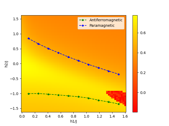
Image Source: \(^{[1]}\)
Stabilizer Codes
QEC is crucial for protecting quantum information from background noise and gate errors that occur during processing. To achieve this, error correction protocols redundantly encode logical qubits into many physical qubits, some of which are ancilla qubits, to ensure errors can be detected and corrected. The ancilla qubits in a stabilizer code are repeatedly measured by parity check operators so that the wavefunction of the state of the logical qubits is not collapsed. The syndrome information is then used to detect and possibly correct errors that are believed to have occurred during processing.
The number of errors that can be detected and corrected is dependent on the code. An \([[n,k,d]]\) QEC code encodes \(k\) logical qubits into a QEC codeword of length \(n\) to protect the system during quantum processing, where the code distance \(d\) determines the minimum number of physical qubit errors needed to cause a logical error. A code of distance \(d\) can correct up to \(\left\lfloor\frac{d-1}{2}\right\rfloor\) errors and detect up to \(d-1\) errors.
The information protected by the stabilizer code is defined over a stabilizer group \(\mathcal{S}\), which is the Abelian subgroup of the Pauli group \(P^{\otimes n}\). This group does not include \(-I^{\otimes n}\), where \(I\) is the \(2\times2\) identity matrix in \(P\). The stabilizer group \(\mathcal{S}\) has \(n-k\) independent generators \(\mathcal{S}_i\), \(i=1,\ldots,n-k\). Each element in the stabilizer group \(\mathcal{S}=\left\langle\mathcal{S}_1,\mathcal{S}_2,\ldots,\mathcal{S}_{n-k}\right\rangle\) is termed a stabilizer. The stabilizer generators perform distinct operations on the data qubits, however all stabilizer generators leave the encoded quantum state unchanged.
Bivariate Bicycle Codes
The BB code is a type of Calderbank-Shor-Steane CSS stabilizer code that leverages bivariate polynomials over the quotient ring \(R=\mathbb{F}_2[x,y]/(x^\ell-1,y^m-1)\), where \(\ell\) and \(m\) are positive integers, and \(\mathbb{F}_2=\{0,1\}\) is the binary field. An \([[n,k,d]]\) BB code \(\operatorname{QC}(A,B)\) is a CSS code defined by two polynomials \(A,B\in R\), where \(\operatorname{QC}(A,B)\) denotes the associated quasi-cyclic code generated by the pair \((A,B)\), and has parameters:
\(n=2\ell m\)
\(k=2\cdot\dim\left(\ker(\mathbf{H}^X)\cap\ker(\mathbf{H}^Z)\right)\)
\(d=\min\left\{|v|:v\in\ker(\mathbf{H}^X)\setminus\operatorname{rs}(\mathbf{H}^Z)\right\}\)
where \(\mathbf{H}^X\) and \(\mathbf{H}^Z\) are the parity-check matrices of the CSS code corresponding to the \(X\)-type and \(Z\)-type stabilizer checks, respectively, and \(\mathbf{H}\) denotes a binary matrix. \(\operatorname{ker}(\mathbf{H})\) denotes the set of vectors orthogonal to each row of \(\mathbf{H}\), \(\operatorname{rs}(\mathbf{H})\) is the linear span of its rows, and \(|v|=\sum_{i=1}^n v_i\) is the Hamming weight of \(v\in\mathbb{F}_2^n\).
Encoding Logical Qubits
The check matrices for a BB code denoted \(\operatorname{QC}(A,B)\) with length \(n=2\ell m\) are:
\(\mathbf{H}^X=[A\mid B]\quad\text{and}\quad\mathbf{H}^Z=[B^T\mid A^T]\)
where the vertical bar indicates stacking matrices horizontally, and \(T\) denotes matrix transpose. The bivariate polynomials are a pair of matrices:
\(A=A_1+A_2+A_3\quad\text{and}\quad B=B_1+B_2+B_3\)
such that each matrix \(A_i\) and \(B_j\) is a power of \(x\) or \(y\), while \(\operatorname{dim}\mathbf{H}^X=\operatorname{dim}\mathbf{H}^Z=(n/2)\times2\). Each row \(v\in\mathbb{F}_2^n\) in \(\mathbf{H}^X\) is an \(X\)-type operator, and similarly each row \(v\in\mathbb{F}_2^n\) in \(\mathbf{H}^Z\) is a \(Z\)-type operator, defined as:
\(X(v)=\prod_{j=1}^n X_j^{v_j}\quad\text{and}\quad Z(v)=\prod_{j=1}^n Z_j^{v_j}\)
respectively. The codes are described using the linear subspace associated with the check matrices and polynomials \(A\) and \(B\) for high rate, shown in \(^{[11]}\) and \(^{[14]}\).
Syndrome Extraction
The standard code \(\operatorname{QC}(A,B)\) has a syndrome measurement SM circuit that continuously measures the syndrome of each check operator, which requires \(n\) data qubits and \(n\) ancillary check qubits to record the measured syndromes, for a total of \(2n\) physical qubits. The SM circuit only applies \(\operatorname{CNOT}\)s to pairs of qubits that are connected in the Tanner graph.
The SM circuit starts and ends with a code dependent initialization and measurement cycle that determines the logical qubit initialization suited for the initial state and measures logical qubits in a proper basis. The rest of the SM circuit is comprised of \(N_c\) syndrome cycles SC repeated throughout the circuit periodically, where each SC measures syndromes for all \(n\) check operators of the code.
Decoding Algorithm
Consider an \([[n,k,d]]\) BB code and an SM circuit \(\mathcal{U}\) constructed with \(N_c\) syndrome cycles. Error correction is performed using a classical algorithm that takes a measured error syndrome as input and returns an estimate of the Pauli error that occurred during computation on the data qubits, accounting for all faults provided by the SM circuit. Note, the syndrome circuit itself may contain measurement errors. A proper guess occurs if the estimated Pauli error is a subset of the actual Pauli error up to a product computed via the check operators.
The SM step is followed by belief propagation with an ordered statistics postprocessing step decoder BP-OSD \(^{[11]}\). The unknown error for the linearized noise model used in the BB code is \(\xi\), \(D\) denotes the decoding matrix, and \(\sigma=\left[s^U\mid s^F\right]\) is the measured error syndrome. Using information sets ranked according to their reliability, BP-OSD finds an information set \(I\) with the largest reliability. The output of BP-OSD is the solution of the system \(D\xi=\sigma\) based on the most reliable information set \(I\). This information set is used as the solution for the minimum weight error \(\xi^*=\xi^*(s)\in\{0,1\}^N\) optimization problem. The guess for the unknown logical syndrome is given as:
\(s^L=D^L\xi^*\)
where \(L\) indexes the logical qubit degree of freedom. The BP-OSD decoder is applied separately to the decoding matrices \(D_x\) and \(D_z\), which are constructed from the parity-check matrices \(\mathbf{H}^X\) and \(\mathbf{H}^Z\), respectively. The result is guessed \(X\)-type and \(Z\)-type errors \(E_x\) and \(E_z\), where the guessed final error is \(E^*=E^*_xE^*_z\). This BP-OSD computes the upper bound for the code distance \(d\).
Error Correction
After executing a quantum circuit, the syndrome measurement outcomes are processed using BP-OSD. The final guessed \(X\)-type error \(E_x\) and \(Z\)-type error \(E_z\) are then used to correct the data qubits without measurement occurring.
Proposed Bivariate-Bicycle Coded QCNN
In this section, we describe the parameters of the distance-\(4\) BB code and the \(4\)-qubit QCNN, followed by a description of how the QCNN is embedded within the BB code using transversal operations, ensuring that all QCNN operations remain within the protected code space. Finally, the Tanner graph topology of the trained network is used to correct errors in the QCNN. The full QEC-QCNN circuit is given as:
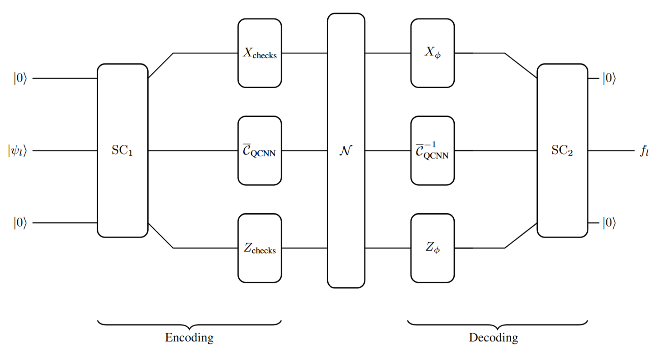
Image Source: \(^{[1]}\)
Training the QCNN
We used the QCNN for quantum phase recognition QPR by applying it to a class of one-dimensional many-body systems. Specifically, the class considered is a \(\mathbb{Z}_2\times\mathbb{Z}_2\) phase. The ground states were numerically obtained using an infinite-size density matrix renormalization group DMRG algorithm, following the method outlined in \(^{[19]}\) with a maximum bond dimension of \(150\). The symmetry operators generating the \(\mathbb{Z}_2\times\mathbb{Z}_2\) symmetry are:
\(X_{\text{even}}=\prod_{i\in\text{even}}X_i\quad\text{and}\quad X_{\text{odd}}=\prod_{i\in\text{odd}}X_i\)
where \(X_i\) is the Pauli-\(X\) operator acting on site \(i\). Each ground state energy density is obtained as a function of \(h_2\) for fixed \(h_1\). We then compute its second-order derivative to locate phase transitions. The QCNN circuit classifies whether the SPT phase exists as an \(|S=1|\) Haldane chain or has transitioned to an \(|S=1|\) paramagnetic phase or antiferromagnetic phase. When \(\omega\) is zero or sufficiently small relative to \(J\), the ground state phase belongs to the SPT phase. The phase is antiferromagnetic when the staggered field \(h_1\) is sufficiently large relative to \(J\), breaking the \(\mathbb{Z}_2\times\mathbb{Z}_2\) symmetry of the SPT phase. The critical point is identified as \(h_2/J=0.423\) using infinite size DMRG numerical simulations.
During training, the untrained model is given a classified training set \(\mathcal{T}_{\text{train}}=\{(|\psi_\alpha\rangle,y_\alpha):\alpha=1,\ldots,M\}\), where \(y_\alpha\) is the respective \(0\) or \(1\) binary classification for some input state \(|\psi_\alpha\rangle\). The expected output of the QCNN is computed as \(f_{\left\{U_i,V_i,F\right\}}\left(\left|\psi_\alpha\right\rangle\right)\). The cost function of the model is computed using the mean-squared error MSE:
\(\texttt{MSE}=\frac{1}{2M}\sum_{\alpha=1}^M\left(y_i-f_{\left\{U_i,V_j,F\right\}}\left(\left|\psi_\alpha\right\rangle\right)\right)^2\)
The QCNN is constructed using isometric tensors in the pooling layer, where measuring a qubit lowers degrees of freedom for feature extraction \(^{[13]}\). Since these measurement-based pooling operations are non-unitary and irreversible, standard quantum backpropagation cannot be applied through the full QCNN. An analytical gradient parameter-shift rule is used as an approximation scheme to compute the gradients, which provides unbiased gradient estimates for the variational unitary layers preceding the measurements.
The model learns by iteratively optimizing all initially assigned unitaries until convergence via a finite-difference scheme given the MSE cost function. To calculate the gradient matrix \(M\) using the finite-difference scheme, the parameterized weights \(\Theta\) in the QCNN circuit are perturbed by shifting \(\theta_j\in\Theta\) by \(\pm\epsilon\) for each parameter in the quantum circuit. The weights are then updated via gradient descent as:
\(\Theta\leftarrow\Theta-\eta\,M\)
where \(\eta\) is the learning rate and \(M\) is the gradient matrix of the MSE with respect to \(\Theta\). We evaluate phase recognition performance using \(40\) spin-\(\frac{1}{2}\) ground states sampled along the \(h_2\) axis with \(h_1=0\), with QCNN weights trained from \(0.616\) to \(0.174\) after \(100\) iterations under ideal, noiseless statevector simulation. The trained model produces expectation values \(\langle Z_m\rangle\) that decrease monotonically from approximately \(0.94\) near \(h_2=0\) toward \(0.28\) at the far end of the paramagnetic region, yielding a smooth decision boundary consistent with the theoretical phase transition at \(h_2/J=0.423\).
Optimizing Quantum Error Correction
The QEC code is a BB code with parameters \([[18,4,4]]\), where \(l=3\) and \(m=3\), using \([a_1,a_2,a_3]=[1,0,1]\) and \([b_1,b_2,b_3]=[2,0,2]\). We derive the corresponding check matrices \(\mathbf{H}^X=[A|B]\) and \(\mathbf{H}^Z=[B^T|A^T]\) and compute the code parameters \(k=4\) and \(d=4\). The BB code circuit is then constructed in accordance with the architecture described in the Bivariate Bicycle Codes section.
The feed-forward correction layer is trained and evaluated on stochastic Pauli noise injected into the \([[18,4,4]]\) BB code. Specifically, the four logical data qubits admit \(2^4=16\) distinct computational basis states, such that the training set is:
\(\mathcal{F}_{\text{train}}=\bigl\{\,y\in\{0,1\}^4\bigr\}\)
where each element \(y=(y_1,y_2,y_3,y_4)\) encodes which of the four logical qubits has suffered a bit-flip error. At each SPSA iteration, every pattern \(y\in\mathcal{F}_{\text{train}}\) is prepared by applying \(X\) gates to the mapped physical qubits. Concretely, the encoder uses the logical map \(\zeta\) to map each basis state \(\lvert y\rangle\), where \(y\in\{0,1\}^4\), to a codeword \(|\overline{y}\rangle\in (\mathbb{C}^2)^{\otimes11}\) via transversal gate operations. Given a physical quantum circuit \(\mathcal{C}\) acting on \(4\) logical qubits, we construct a physically encoded circuit \(\mathcal{C}_{\text{enc}}\) via the transversal gate operations.
Given the logical state space is finite and small, the loss is computed over all \(N=16\) patterns at every iteration, making each update equivalent to a full-batch gradient step over the complete input distribution. This exhaustive evaluation guarantees that the trained parameters \(\vec{\phi}\) are assessed on every failure mode of the code, and that a loss of \(0\) certifies perfect logical-state recovery across all possible single-layer error configurations.
To correct errors, we augment the syndrome extraction circuit with a parametrized feed-forward layer. This layer introduces \(2m\) trainable rotation angles \(\phi_i\in[0,2\pi)\), where \(R_y(\phi_i^X)\) and \(R_y(\phi_i^Z)\) denote single-qubit \(y\)-axis rotation gates parameterized by the \(i\)th trainable angle corresponding to the \(X\)-check and \(Z\)-check ancilla qubits, respectively. These rotations are applied to the physical data qubits immediately following the syndrome vector, using controlled \(X\) and \(Z\) rotations.
The objectives used during training are the logical states, or logical labels. Given the set of true logical labels \(\{y_i\}_{i=1}^{N}\) and the corresponding predicted logical labels \(\{\hat{y}_i\}_{i=1}^{N}\) returned by the decoder after circuit execution, the loss is given as:
\(\texttt{Loss}(\vec{\phi})=\frac{1}{N}\sum_{i=1}^{N}\mathbf{1}\!\left[\hat{y}_i\neq y_i\right]\)
where \(\vec{\phi}\) denotes the trainable parameters of the QEC feed-forward layer, distinct from the QCNN circuit parameters \(\vec{\theta}\), and \(\mathbf{1}[\cdot]\) denotes the indicator function. The loss therefore lies in \([0,1]\), with \(0\) indicating perfect correction and \(1\) indicating every frame is mislabeled. This normalization gives the SPSA gradient estimator a stationary, bounded signal that is independent of the number of test cases and the code distance.
The correction layer is embedded inside a quantum circuit evaluated by a noisy stochastic simulator. Since the loss function is a non-differentiable indicator function, gradients of \(\texttt{Loss}\) with respect to the trainable parameters \(\vec{\phi}\) cannot be computed analytically \(^{[20]}\). SPSA is therefore employed as the optimizer, such that at each iteration \(k\) the algorithm evaluates a single syndrome cycle circuit \(3\) times, regardless of the number of parameters \(p\), making it practical for circuits with many syndrome checks. Each training iteration proceeds in four stages: center evaluation, positive perturbation, negative perturbation, and the gradient step.
For the center evaluation, the unperturbed circuit is evaluated to obtain the center-point loss \(\texttt{Loss}_0=\texttt{Loss}(\vec{\phi}^{(k)})\), where \(\vec{\phi}^{(k)}\) is the weight vector at the \(k\)th iteration. For the positive perturbation, a simultaneous perturbation vector \(\vec{\Delta}\in\{-1,+1\}^p\) is drawn independently and uniformly at random, the parameters are shifted to \(\vec{\phi}^{(k)}+c\,\vec{\Delta}\), where \(c=0.2\) rad is the perturbation magnitude, and the circuit is evaluated to obtain \(\texttt{Loss}_+\). For the negative perturbation, the parameters are shifted to \(\vec{\phi}^{(k)}-c\,\vec{\Delta}\) using the same realization of \(\vec{\Delta}\), and the circuit is evaluated to obtain \(\texttt{Loss}_-\).
For the gradient step, the SPSA gradient estimate for parameter \(i\) is:
\(\hat{g}_i=\frac{\texttt{Loss}_+-\texttt{Loss}_-}{2\,c\,\Delta_i}\)
and a gradient descent step is applied:
\(\phi_i^{k+1}=\left(\phi_i^{k}-\alpha_k\,\hat{g}_i\right)\!\!\mod2\pi\)
where \(\alpha_k\) is the current learning rate. All parameters are updated simultaneously in a single step, with the base parameters restored from a snapshot taken before the perturbations were applied. Angles are wrapped modulo \(2\pi\) throughout.
The learning rate \(\alpha_k\) is adapted at every step by a bold-driver rule \(^{[21]}\). After the gradient step, the center-point loss \(\texttt{Loss}_0\) of the current iteration is compared against that of the previous iteration. If the loss has decreased, then the learning rate is increased by \(1.05\), encouraging larger steps when progress is being made. If the loss has increased or remained constant, the learning rate is halved, contracting the search radius to:
\(\alpha_{k+1}=\begin{cases}1.05\,\alpha_k&\text{if }\texttt{Loss}_0^{(k)}\lt\texttt{Loss}_0^{(k-1)},\\0.5\,\alpha_k&\text{otherwise.}\end{cases}\)
All trainable parameters are initialized to zero, corresponding to identity rotations on every check qubit. Under this initialization the correction layer has no effect on the circuit output, so the very first center-point evaluation measures the uncorrected logical error rate. Subsequent iterations introduce progressively stronger corrections as SPSA explores the parameter space. A seeded random number generator is used for both the initialization procedure and the Bernoulli draws that produce the \(\vec{\Delta}\) vectors, ensuring that training runs are exactly reproducible.
Error Correction for QCNN
The QCNN suffers from the error-prone nature of quantum operations throughout the entirety of the circuit, so it naturally motivates the need for QEC. Our proposed QCNN architecture constructs the layers using transversal gate operations that conform to the Tanner graph structure of the BB code, denoted \(\overline{\mathcal{C}}_{\text{QCNN}}\). This allows gates in each layer to preserve the code's locality and operations to occur in the protected subspace. The variational parameters are continuous and therefore implement non-Clifford rotations, which cannot be implemented transversally in the BB data block, allowing for errors to propagate through the circuit.
To mitigate this, while avoiding the high overhead of magic state injection MSI, we employ an FFNN as a syndrome-based neural decoder interleaved between each convolutional, pooling, and fully connected layer of the QCNN and the next. Thus, rather than correcting the non-Clifford rotations themselves, the FFNN intercepts the \(X\)-syndromes and \(Z\)-syndromes produced by the BB code's stabilizer checks after each noisy layer, and predicts per-qubit Pauli-\(X\) and Pauli-\(Z\) correction decisions before the next layer executes. This approach confines error propagation to within individual layers rather than allowing it to compound across the full circuit depth.
Concretely, this correction occurs between each hidden layer, prior to the next variational layer, so that the parameter updates computed by SPSA reflect gradient estimates over a cleaner logical state rather than one corrupted by accumulated gate noise, as would occur if correction were deferred to end-of-circuit. This process circumvents the classical post-processing bottleneck of BP-OSD, where belief propagation would need to complete on the order of \(1\mu s\) \(^{[22]}\), \(^{[23]}\) for superconducting processors to keep pace with circuit execution. Current state-of-the-art decoders trade accuracy for latency to meet this tight decoding time budget \(^{[24]}\), and BP-OSD does not meet this requirement at scale. Otherwise, physical qubits must sit idle between layers, during which \(T_1\) energy relaxation and \(T_2\) dephasing processes accumulate additional errors on the quantum hardware.
The FFNN's learnable weights are one per edge of the BB code's Tanner graph, such that the structure of the check and variable nodes respects the code's locality, mirroring the same geometric constraints imposed on the transversal gates. Its input is the \(X\)-syndrome bit string extracted from stabilizer \(\operatorname{CX}\) measurements on the \([[18,4,4]]\) BB code's ancilla qubits, and its output is a binary correction vector indicating which physical data qubits require a corrective \(\operatorname{CX}\) operation to return the logical state to the code space.
The \(4\)-spin SPT input state is encoded into an \(18\)-physical-qubit state representing the logical state \(|\psi_l\rangle\) of the \([[18,4,4]]\) code. The encoding is performed by mapping the four physical input spins to logical qubit degrees of freedom according to the sparse parity-check structure of the code. For each logical circuit \(\mathcal{C}\), this procedure traverses every layer of the QCNN, including the input layer and final layer. The transversal operations then replace each logical instruction with up to \(|\mathcal{P}_c|\times|\mathcal{P}_t|\) physical gates. For a code with block size \(n\) and a circuit of depth \(d\) containing \(g\) two-qubit gates, the encoded circuit has depth at most \(\mathcal{O}(d)\) and gate count at most \(\mathcal{O}(g\cdot n^2)\). Specifically, each gate \(G\in\mathcal{C}\) acting on logical qubit \(q_i\) is replaced by the transversal operation:
\(G^{\otimes|\mathcal{P}_i|}=\bigotimes_{j\in\mathcal{P}_i}G_j\)
where \(\mathcal{P}_i\subseteq\{0,1,\ldots,n-1\}\) is the set of physical qubit indices corresponding to the \(i\)th logical qubit under the code's qubit mapping \(\zeta:q_i\mapsto \mathcal{P}_i\). A logical CNOT between control qubit \(q_c\) and target qubit \(q_t\) is implemented transversally as:
\(\mathrm{CNOT}^{\otimes}=\bigotimes_{\substack{j\in\mathcal{P}_c\\k\in\mathcal{P}_t,\;j\neq k}}\mathrm{CNOT}_{j\to k}\)
applying a physical CNOT from each control physical qubit to each target physical qubit, excluding self-connections. Gates involving stabilizer check qubits or reset operations are passed through without transversal expansion, as these are already defined at the physical level in the encoded circuit.
The \(\overline{\mathcal{C}}_{\text{QCNN}}\) then acts on the logical state, which undergoes noise \(\mathcal{N}\) as:
\(f_l=\sum_{\lvert\psi_l\rangle\in\{\lvert{\pm x,y,z}\rangle\}}\langle\psi_l\rvert\,\mathcal{M}_q^{-1}\!\left(\mathcal{N}\!\left(\mathcal{M}_q\!\left(\lvert\psi_l\rangle\langle\psi_l\rvert\right)\right)\right)\lvert\psi_l\rangle\)
where \(\mathcal{M}_q\) and \(\mathcal{M}_q^{-1}\) denote the encoding and decoding maps of the BB code, \(\lvert{\pm x,y,z}\rangle\) are the \(\pm1\) eigenstates of the Pauli \(X\), \(Y\), \(Z\) operators, and \(f_l\) is the logical output of \(\overline{\mathcal{C}}_{\mathrm{QCNN},\,\{U_i,\,V_j,\,F\}}\!\left(\lvert\psi_l\rangle\right)\).
The initial physical system has two \(9\)-qubit data registers \(\mathcal{D}_L\) and \(\mathcal{D}_R\), one \(9\)-qubit \(X\)-check ancilla register \(\mathcal{A}_X\), and one \(9\)-qubit \(Z\)-check ancilla register \(\mathcal{A}_Z\). However, the transversal qubit mapping makes the two data registers redundant. The four logical qubits map onto only \(11\) distinct physical qubit indices \(\{0,\ldots,10\}\), with qubits \(\{0,2,5,6\}\) shared across multiple logical qubits and the remaining indices each carrying information unique to a single logical qubit. Consequently, the two data registers collapse into a single \(11\)-qubit register \(\mathcal{D}\), reducing the full system from \(36\) to \(29\) qubits without loss of information.
The evolved circuit is a Hilbert space of dimension \(2^{n_\text{total}}\), where \(n_\text{total}=n_\text{left}+d_\text{data}+n_\text{right}=29\), given \(9\) \(X\)-check ancillas, \(11\) data qubits, and \(9\) \(Z\)-check ancillas. Given the ancilla qubits are initialized to \(|0\rangle\) and, in the noiseless statevector simulation, remain unentangled with the data register, the data-qubit marginal state can be extracted without a partial trace. The reduced statevector is then decoded into the logical basis by iterating over all \(2^{d_\text{data}}\) computational basis states of the data register. The corresponding logical state is then determined by:
\(\mathbf{v}=\left[\,\bigl(L_X\,\mathbf{b}\bigr)\bmod2\,\right]\)
The complex amplitude \(\alpha_j\) is then accumulated into the entry of the logical statevector \(|\psi_l\rangle\in\mathbb{C}^{2^N}\) indexed by \(v=\sum_k v_k\,2^{N-1-k}\), so that:
\(|\psi_l\rangle=\sum_{j=0}^{2^{d_\text{phys}}-1}\alpha_j\,\bigl|\mathbf{v}(\mathbf{b}_j)\bigr\rangle\)
The resulting \(2^{N}\)-dimensional statevector is passed to the prediction stage, where the expectation value of the middle-qubit observable is evaluated to produce the final classification output.
Experimental Results and Discussion
Simulation Setup
We let each gate type be subject to an independent error probability \(p\), with errors injected as single- or two-qubit Pauli operators drawn uniformly from \(\{I,X,Y,Z\}\). The two-qubit CNOT gates are assigned errors from the full \(15\)-element two-qubit Pauli group \(\{I,X,Y,Z\}^{\otimes2}\setminus\{II\}\), with each error type drawn uniformly given that an error occurs with probability \(p\). Idle qubit errors are inserted to maintain a consistent time boundary across all data qubits. Idle qubits are modeled per layer, such that any qubit not involved in an active gate receives a uniformly random Pauli error \(\{I,X,Y,Z\}\) with probability \(p\), independently per qubit. Measurement operations are subject to a pre-measurement bit-flip, phase-flip, or \(Y\)-error at the same rate.
Further, we implement a stochastic Pauli noise model applied at the circuit level \(^{[11]}\). The considered noise model configuration is used to sweep over physical error rates \(p\in\{0.0001,0.001,0.003\}\), which span the near-threshold regime relevant to NISQ-era demonstrations. This noise model approximates a symmetric depolarizing channel on each gate type and serves as a baseline for evaluating the robustness of our BB-code- protected QCNN against gate-level noise. All noise simulations used the same seeded random number generator for reproducibility.
Training and Evaluation
The \(4\)-qubit QCNN was first trained under ideal statevector simulation using a dataset of \(40\) labeled ground states evenly spaced along the line \(h_2=0\), where the Hamiltonian is exactly solvable via the Jordan-Wigner transformation and labeled \(\pm1\) \(^{[25]}\). Training ran for \(100\) iterations using the finite-difference gradient scheme. The statevector training loss for the \(4\)-qubit QCNN and the \(11\)-qubit transversal QCNN under error rates \(p\in\{0.0\)%\(,0.01\)%\(,0.1\)%\(,0.3\)%\(\}\) is given below.
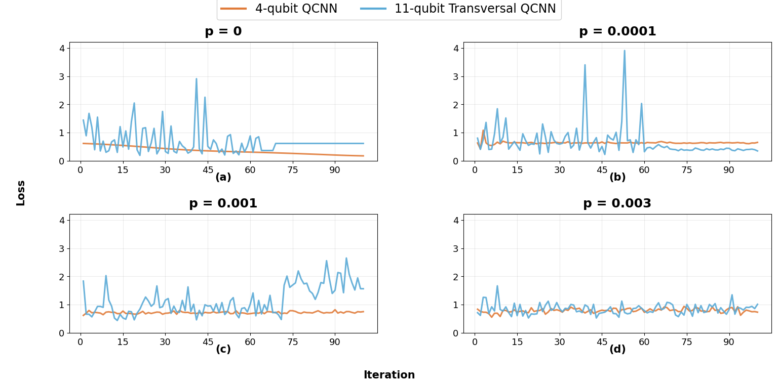
Image Source: \(^{[1]}\)
Under noiseless conditions, that is \(p=0\), statevector training shows the standard QCNN converging smoothly and monotonically from \(0.616\) to \(0.174\), reaching a stable plateau by iteration \(60\). In comparison, the transversal QCNN started at \(1.442\) and exhibits substantial loss variance during the first \(55\) iterations, with a quick peak exceeding \(2.0\) and recurring peaks near iterations \(20\) and \(45\). After iteration \(55\), the transversal circuit stabilizes and plateaus at \(0.616\), with the lowest loss at iteration \(19\) of \(0.19\) and oscillating around losses of about \(0.25\) from iterations \(20\) to \(60\).
This variability and performance gap of the transversal QCNN under noiseless conditions suggest structural constraints due to the transversal gate set. We believe that the application of an identical unitary operation fault-tolerantly across all physical qubits reduces the effective expressibility of the ansatz. Updates made to the weights are magnified by the repetition of the gates across many physical qubits. While this property is designed to minimize physical error rates on a logical qubit, it also causes large shifts for the finite-difference scheme when traversing the gradient. This can be seen by the large steps taken during early training, before plateauing after the learning loss was lowered, due to fine tuning from the bold driver.
For \(p=0.001\), the standard QCNN fails to learn and converge entirely. The loss starts at \(0.632\) and after \(100\) iterations is at \(0.652\). The QCNN reaches its lowest loss of \(0.42\) at iteration \(2\), after which it never drops below a loss of \(0.6\). The transversal QCNN starts at \(0.802\) and oscillates early on, however it starts learning and descending around iteration \(45\), ending at \(0.348\). The lowest loss recorded for the transversal QCNN was \(0.224\) at iteration \(46\). Given the transversal QCNN learned better than the standard QCNN without noise, we believe the error corrected QCNN will train better, however, with limited hardware, we leave simulating \(29\) qubits on classical hardware for future research.
For \(p=0.003\), the highest noise level tested for training, the standard QCNN begins at a loss of \(0.714\) at iteration \(1\) and never improves in any sustained amount. We assume this is because the bold-driver schedule triggers repeated halving events from as early as iteration \(3\), collapsing the learning rate from \(10^5\) to below \(10^{-8}\) by iteration \(100\), at which point the loss reads \(1.565\), higher than the starting loss.
At the same error rate, the transversal QCNN follows a similar loss volatility but exhibits markedly higher loss magnitudes throughout. The initial loss started at \(0.714\) at iteration \(1\), and the model oscillates chaotically across the full \(100\) iterations, with losses regularly exceeding \(1.0\) and peaking above \(1.6\) at iterations \(8\) and \(38\), respectively. The learning rate undergoes the same rapid collapse as the standard variant, falling below \(10^{-8}\) before iteration \(100\), and the final loss of \(1.565\) provides no improvement over initialization. Neither architecture recovers a downward trend after the learning rate saturates near zero, and neither approaches the \(0.348\) final loss achieved by the transversal QCNN at \(p=0.001\). This shows that an error rate of \(p=0.003\) is too high for the trainability of both the standard and transversal QCNN under the present finite-difference scheme configuration.
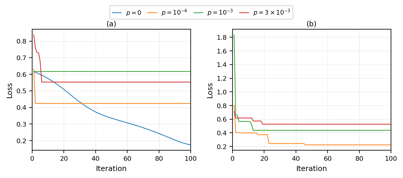
Image Source: \(^{[1]}\)
Above, the best-so-far training loss over \(100\) iterations is plotted for the standard QCNN and the transversal QCNN under different NISQ noise levels \(p\in\{0,0.0001,0.001,0.003\}\). Each plotted value reflects the lowest loss achieved up to that iteration rather than the raw per-iteration loss. Under noiseless conditions, the standard QCNN converges smoothly and monotonically to a final loss of approximately \(0.174\), whereas all noisy variants stall early, with \(p=0.001\) and \(p=0.003\) plateauing immediately near \(0.62\) and \(0.57\) respectively, and \(p=0.0001\) halting around \(0.43\) after a few iterations. All four noise levels for the transversal QCNN descend rapidly within the first \(10\) iterations and continue improving, with the noiseless curve reaching approximately \(0.21\), \(p=0.0001\) settling near \(0.22\), and even the noisiest conditions converging to losses of roughly \(0.43\) and \(0.50\) respectively. This contrast demonstrates that the transversal architecture retains trainability at noise levels that completely suppress learning in the standard QCNN.
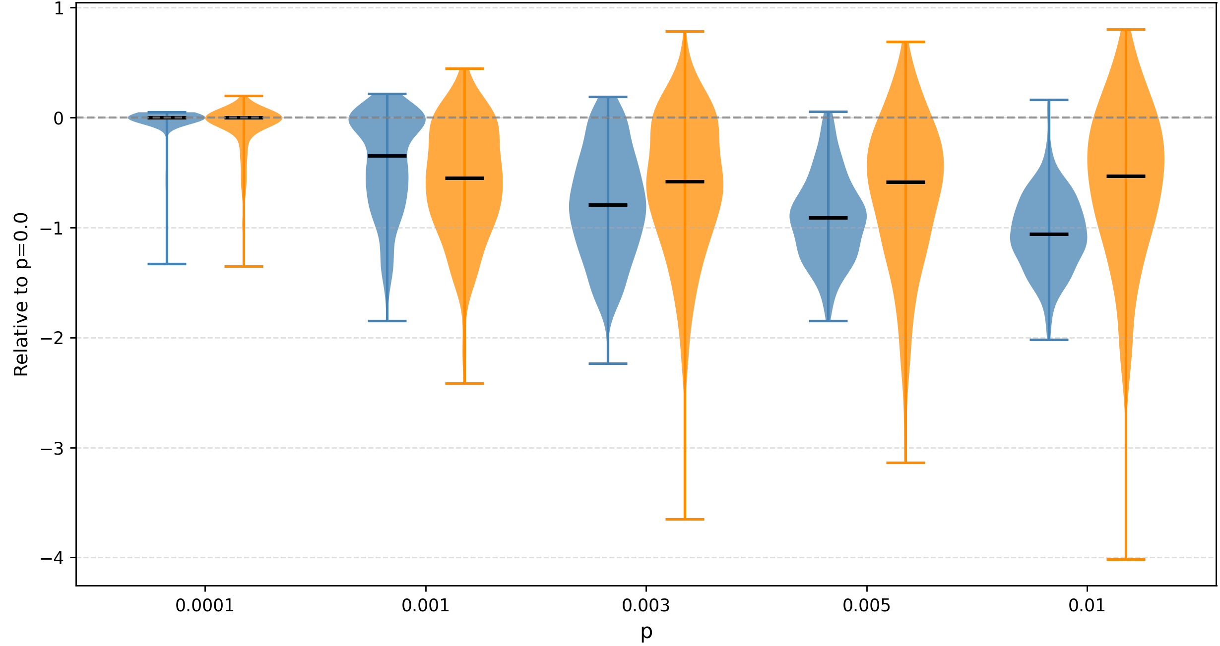
Image Source: \(^{[1]}\)
The violin plots above show qubit prediction values for the standard QCNN and logical prediction values for the transversal QCNN across Pauli noise levels, normalized to the noise-free statevector predictions. Each noise level has \(n=50\) predictions over \(25\) random seeds. At \(p=0.0001\), both architectures remain tightly concentrated near zero, indicating minimal deviation from the noiseless baseline. As noise increases to \(p\geq0.001\), both distributions shift downward and broaden, reflecting degraded and increasingly variable predictions. The standard QCNN consistently produces a more compact and symmetric distribution with its median tracking closer to zero at lower noise levels, reaching approximately \(-1.05\) at \(p=0.005\) and \(-1.2\) at \(p=0.01\).
The transversal QCNN, by contrast, exhibits wider distributions with heavier tails extending well below \(-2\) at higher noise levels, and while its median remains slightly higher than the standard QCNN at \(-0.7\) and \(-0.6\) for \(p=0.005\) and \(p=0.01\) respectively, this comes with substantially greater variance and outliers. We can conclude that the transversal gate structure preserves higher median prediction quality at elevated noise levels at the cost of greater variance, and that this preservation of median predictions may allow the optimizer to identify clearer local minima during noisy training.
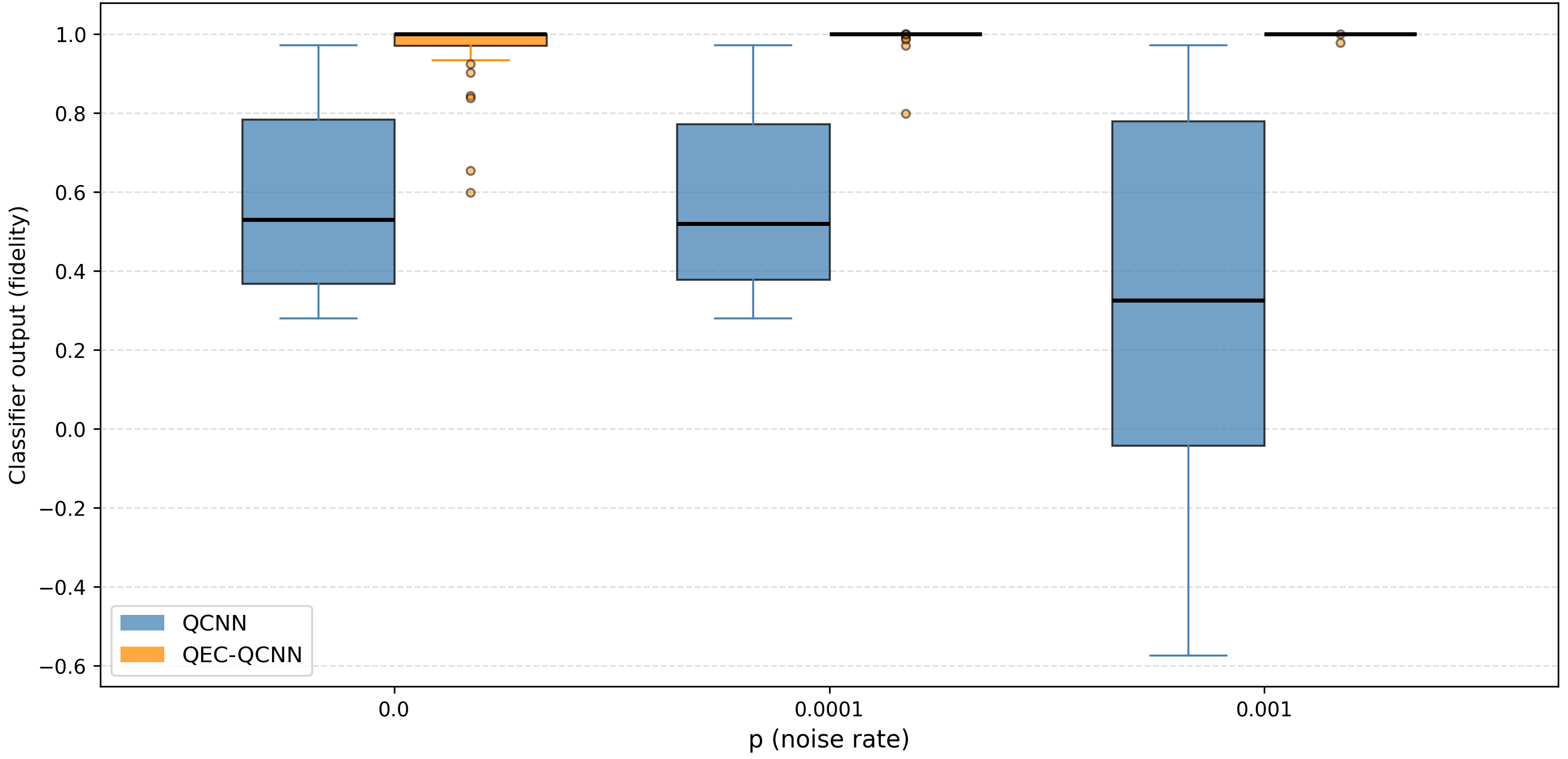
Image Source: \(^{[1]}\)
The QEC-QCNN results above show that the FFNN trained on Clifford gates over corrects for errors. Non-Clifford gates are not a part of the training data, and appear to the FFNN soft decoder as errors. This causes bit and phase flips to the entangled data, causing predictions to entropy to predictions of \(1\). To improve results, the FFNN soft decoder should be trained with the QCNN model, for noise-aware error correction, or trained on a pre-trained model. Thus, errors in application match errors seen during training.
Qubit Resource Analysis
The toric surface code encodes logical qubits into a physical qubit lattice with overhead scaling as \(n\propto d^2\), achieving an error threshold of approximately \(0.67\)%-\(0.81\)% under circuit-level depolarizing noise using gauge-fixing techniques \(^{[26]}\), below which increasing \(d\) exponentially suppresses logical errors. However, encoding \(k=4\) logical qubits at distance \(d=4\) requires roughly \(64\) physical qubits plus \(400\)-\(1{,}000\) additional qubits per magic state distillation factory \(^{[27]}\), \(^{[28]}\) to supply the non-Clifford gates essential to QCNN variational layers at current gate error rates \(^{[29]}\), placing total physical qubit requirements between \(10^4\) and \(10^6\) \(^{[30]}\), \(^{[31]}\), \(^{[32]}\). This is a prohibitive overhead for current hardware.
By contrast, the \([[18,4,4]]\) BB code encodes the same \(4\) logical qubits into \(29\) physical qubits via a shared-index transversal mapping, with non-Clifford corrections handled by the interleaved FFNN decoder, eliminating factory overhead at the cost of a lower error threshold of about \(0.3\)%. This makes it far better suited to near-term operation.
Conclusion and Future Directions
In this study, we considered the problem of training instability of the QCNN observed under NISQ hardware noise. We proposed the integration of the BB code to overcome this issue. The \([[18,4,4]]\) BB code provides a mapping for physical to logical qubits and spins via the sparse parity check matrices to transversally encode a \(4\)-qubit QCNN into an \(11\)-qubit QCNN logical structure. The transversal QCNN retains meaningful learning progress at \(p=0.001\) and converges to a final loss of \(0.348\), demonstrating that fault-tolerant encoding confers measurable noise resilience even without a fully trained decoder.
At higher noise rates, such as \(p=0.003\), neither architecture recovers. This indicates that the gradient landscape is too difficult for current QCNN models without meaningful error correction. These findings necessitate joint error mitigation and error correction between the FFNN soft decoder and the transversal QCNN. When higher qubit counts become available, qLDPC codes with larger distances and more logical qubits can be applied to deeper QCNN models. Further, by co-training the decoder alongside the QCNN variational parameters, or by initializing from a pre-trained QCNN model, the correction layer can be exposed to the same error distribution encountered during inference, aligning the noise seen at training time with that seen in application.
References
\(^{[2]}\) S. Hochreiter, "The vanishing gradient problem during learning recurrent neural nets and problem solutions," International Journal of Uncertainty, Fuzziness and Knowledge-Based Systems, vol. 6, no. 2, pp. 107-116, 1998.
\(^{[3]}\) R. Pascanu, T. Mikolov, and Y. Bengio, "On the difficulty of training recurrent neural networks," in Proceedings of the 30th International Conference on Machine Learning, 2013.
\(^{[4]}\) H.-Y. Huang, R. Kueng, and J. Preskill, "Information-theoretic bounds on quantum advantage in machine learning," Physical Review Letters, vol. 126, no. 19, p. 190505, 2021.
\(^{[5]}\) M. A. Nielsen and I. L. Chuang, Quantum Computation and Quantum Information: 10th Anniversary Edition. Cambridge, U.K.: Cambridge University Press, 2011.
\(^{[6]}\) M. Hirvensalo, Quantum Computing, 2nd ed. Berlin, Germany: Springer, 2001.
\(^{[7]}\) J. Biamonte, et al., "Quantum machine learning," Nature, vol. 549, pp. 195-202, 2017.
\(^{[8]}\) V. Havlíček, et al., "Supervised learning with quantum-enhanced feature spaces," Nature, vol. 567, pp. 209-212, 2019.
\(^{[9]}\) J. M. Gambetta, J. M. Chow, and M. Steffen, "Building logical qubits in a superconducting quantum computing system," npj Quantum Information, vol. 3, pp. 1-7, 2017.
\(^{[10]}\) A. Y. Kitaev, "Fault-tolerant quantum computation by anyons," Annals of Physics, vol. 303, no. 1, pp. 2-30, 2003.
\(^{[11]}\) S. Bravyi, A. W. Cross, J. M. Gambetta, et al., "High-threshold and low-overhead fault-tolerant quantum memory," Nature, vol. 627, pp. 778-782, 2024.
\(^{[12]}\) D. Gottesman, "Fault-tolerant quantum computation with constant overhead," Quantum Information and Computation, vol. 14, no. 15-16, 2014.
\(^{[13]}\) I. Cong, S. Choi, and M. D. Lukin, "Quantum convolutional neural networks," Nature Physics, vol. 15, no. 12, pp. 1273-1278, Dec. 2019.
\(^{[14]}\) K. Wang, Z. Lu, C. Zhang, et al., "Demonstration of low-overhead quantum error correction codes," Nature Physics, vol. 22, pp. 308-314, 2026.
\(^{[15]}\) P. Bermejo, et al., "Quantum convolutional neural networks are effectively classically simulable," PRX Quantum, vol. 7, no. 2, p. 020304, Apr. 2026.
\(^{[16]}\) Y. LeCun, Y. Bengio, and G. Hinton, "Deep learning," Nature, vol. 521, no. 7553, pp. 436-444, May 2015.
\(^{[17]}\) Y. LeCun and Y. Bengio, "Convolutional networks for images, speech, and time-series," in The Handbook of Brain Theory and Neural Networks, 1995.
\(^{[18]}\) D. Pomarico, "Multiscale entanglement renormalization ansatz: Causality and error correction," Dynamics, vol. 3, no. 3, pp. 622-635, 2023.
\(^{[19]}\) I. P. McCulloch, "Infinite size density matrix renormalization group, revisited," arXiv preprint arXiv:0804.2509, 2008.
\(^{[20]}\) J. C. Spall, "Multivariate stochastic approximation using a simultaneous perturbation gradient approximation," IEEE Transactions on Automatic Control, vol. 37, no. 3, pp. 332-341, 1992.
\(^{[21]}\) R. Battiti, "First- and second-order methods for learning: Between steepest descent and Newton's method," Neural Computation, vol. 4, no. 2, pp. 141-166, Mar. 1992.
\(^{[22]}\) Google Quantum AI and Collaborators, "Quantum error correction below the surface code threshold," Nature, vol. 638, pp. 920-926, 2025.
\(^{[23]}\) L. Caune, et al., "Demonstrating real-time and low-latency quantum error correction with superconducting qubits," arXiv preprint arXiv:2410.05202, 2024.
\(^{[24]}\) J. Viszlai, et al., "Low latency GNN accelerator for quantum error correction," arXiv preprint arXiv:2603.22149, 2025.
\(^{[25]}\) S. Sachdev, Quantum Phase Transitions, 2nd ed. Cambridge, U.K.: Cambridge University Press, 2011.
\(^{[26]}\) O. Higgott and N. P. Breuckmann, "Subsystem codes with high thresholds by gauge fixing and reduced qubit overhead," Physical Review X, vol. 11, no. 3, 2021.
\(^{[27]}\) D. Litinski, "Magic state distillation: Not as costly as you think," Quantum, vol. 3, p. 205, Dec. 2019.
\(^{[28]}\) B. Eastin and E. Knill, "Restrictions on transversal encoded quantum gate sets," Physical Review Letters, vol. 102, no. 11, p. 110502, 2009.
\(^{[29]}\) IBM Quantum, "IBM Quantum delivers on 2022 100×100 performance challenge," IBM Quantum Blog, Nov. 2024. [Online]. Available: https://www.ibm.com/quantum/blog/qdc-2024
\(^{[30]}\) C. Gidney and M. Ekerå, "How to factor 2048 bit RSA integers in 8 hours using 20 million noisy qubits," Quantum, vol. 5, p. 433, 2021.
\(^{[31]}\) J. Lee, et al., "Even more efficient quantum computations of chemistry through tensor hypercontraction," PRX Quantum, vol. 2, p. 030305, 2021.
\(^{[32]}\) R. Babbush, J. R. McClean, M. Newman, C. Gidney, S. Boixo, and H. Neven, "Focus beyond quadratic speedups for error-corrected quantum advantage," PRX Quantum, vol. 2, p. 010103, 2021.