Information Theory
Quantities of Information
Shannon Information
Three properties were required by Shannon:
- \(I(p) \geq 0\), i.e. information is a real non-negative measure.
- \(I(p_{1},p_{2})=I(p_{1})+I(p_{2})\) for independent events.
- \(I(p)\) is a continous function of \(p\).
The mathematical function that satisfies these requirements is:
\(I(p)=k\;log(p)\)
In the equation, the value of \(k\) is arbitrary, so we choose \(k=-1\) to make the math more convient.
\(I(p)=-\log(p)=\log(\frac{1}{p})\)
The base of the logarithm is representative of the units of measure for the given information, but can also be chosen arbitarily. However, today units of information are exclusively use base 2 logarithms, in units of bits.
\(I(p)=-\log_{2}(p)=\log_{2}(\frac{1}{p})\) bits of information.
Shannon Entropy and Average Code Length
Let \(S=\left\{s_{1}, s_{2},\ldots s_{n}\right\}\) some information source with \(n\) symbols. Let \(P=\left\{p_{1}, p_{2}, \ldots p_{n}\right\}\) be the corresponding probability distribution.
Entropy of the source is the defined as:
\(H(S)=-\sum_{i=1}^{n}p_{i}\log_{2}(p_{i})\)
\(=\sum_{i=1}^{n}p_{i}\log_{2}\frac{1}{p_{i}}\)
Another important number is the average code length \(L_{avg}\), defined as:
\(L_{avg}=\sum_{i=1}^{n}p_{i} \left(\lceil\log_{2}\frac{1}{p_{i}}\rceil+1\right)\)
Where, \(c_{i}\) is some code string of the code set \(C\) and \(|\;|\) is the cardinality of \(c_{i}\).
Note, the entropy of the source is a lower bound on the average code length that can be achieved, given by \(H(S) \leq L_{avg}\). Meaning, that the source entropy can be reach the compression limit, but can never exceed it.
Kraft Inequality
\(K=\sum_{i=1}^{q}\frac{1}{r^{l^{i}}}\leq 1\)
Where:
- \(K\) is the Kraft sum
- \(q\) is the number of source symbols
- \(r\) is the radix of the channel alphabet
- \(l_{i}\) is the lengths of the coded symbols.
Note that the craft inequality must be satisfied for codes that called uniquely decodable, instantaneous codes, or prefix-free codes.
Proof of Achieving Entropy Bound
We can prove the entropy bound that can be achieved using a sufficiently large extension. We can first define that:
\(H(S)\leq L_{avg} < H(S)+1\)
We take the extension for any code to the \(n^{th}\) term, resulting in:
\(H(S^{n})\leq L_{n} < H(S^{n})+1\)
We sequence \(n\) symbols from \(S\), taken from the extended source \(S^{n}\), which now has \(q^{n}\) symbols.
Lastly, we divide our previous equation by \(n\), giving us:
\(H(S)\leq \frac{L_{n}}{n} < H(S)+\frac{1}{n}\)
What this shows, is that by choosing \(n\) sufficently large, the average code length can come arbitrarily closer to source entropy, \(H(S)\).
This being said, there are practical limitations to choosing a large extension on our source symbols. As the extensions on our souce become larger, the returns on efficecny deminish and have a higher cost on delay, stroage, and computation.
System Entropies
The system entropies represent the input and output entropies. The source entropy can be defined as:
\(H_{r}(A)=\sum_{i=1}^{q}p(a_{i})\log_{r}\left(\frac{1}{p(a_{i})}\right)\)
Recall that properties of the entropy function are:
- \(H_{r}(A)\geq 0\)
- \(H_{r}(A)\leq \log_{r}q\), where \(q\) is the number of input symbols
- \(H_{r}(A)=\log_{r}q\) when all source symbols are equally likely
The output entropy can be defined as:
\(H_{r}(B)=\sum_{j=1}^{s}p(b_{j})\log_{r}\left[\frac{1}{p(b_{j})}\right]\)
Conditional Entropy
To continue.
Mutual Information
To continue.
Channel Capacity
To continue.
Hamming Code and Error Correcting
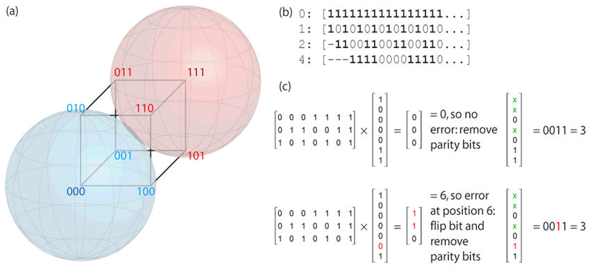
We will look at the encoding of a binary source for transmission on a noisy channel and then build a Hamming Code to transmit one bit of information. The Hamman Coding Model illustrated below shows two valid codewords spheres in \(3\)-dimensional Hamming Space:
Mathematical Tools
Hamming Distance
Given two \(N\)-bit binary symbols, the Hamming distance between them is the number of symbols that differ. For example, if the symbols are \(0110\) and \(1010\) is \(2\).
Note, that binary numbers can be represented as points in an \(N\)-dimensional Hamming Space.
N-Dimensional Hamming Space
The volume of an \(N\)-dimensional Hamming space is based on the number of binary numbers or points in the \(N\)-bit binary number and is defined as \(2^{N}\). The hamming space is represented with a set of \(N\) coordinate axes, where each axis contains the discrete values \(\left\{0,1\right\}\).
The figure below is an example of \(N=4\) dimensional space cube representing a \(4\)-dimensional Hamming space.
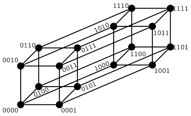
Hamming space gets harder to visualize when the number of dimensions gets larger, but we must trust the math.
Encoding Source Symbols
Let us look at a \(3\)-dimensional Hamming space for the encoding of a binary source on a noisy channel to help us understand encoding source symbols.
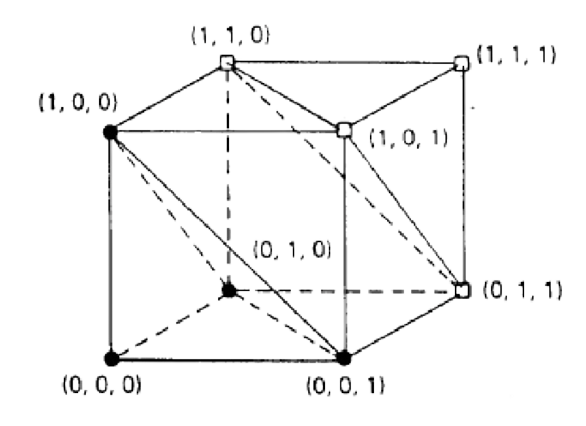
Image Source: Methods of Mathematics Applied to Calculus, Probability, and Statistics by Richard Wesley Hamming
Let the source alphabet be \(\left\{s_{0}, s_{1}\right\}\) with triple repetition coding \(s_{0}=000, s_{1}=111\).
Encoding a binary source for transmission over a noisy channel can cause bit error, so the decoder needs to try to catch and fix this. To do, the decoder will map the recievecd codeword to the closest legal coderword, which is smallest Hamming distance. By looking at our \(3\)-dimensional Hamming space, we can see that the encoder needs to encode the source symbols by a sequence of channel symbols with a "good" distance. This allows for the decoder to have an eaiser time catching and correcting bit errors. However, the decoder can still be foolder by multiple bit errors.
Hamming Distance of a Code
The Hamming distance of a code can be defined as the minimum pairwise Hamming distance between all of the codeword pairs and can allows us to measure the error correction capability of a code.
Given a Hamming code in \(3\)-dimensional Hamming space, there exists a subset of points in that is the set of legal codewords. To optimize error correction capability of a code, we need to spread out the set of legal codewords in \(3\)-dimensional space such that they all have the maximum possible mututal Hamming distances.
Hamming Code
Hamming Codes
Hamming codes are a family of perfect single error correcting codes that can correct all \(1\)-bit errors or detect all \(2\)-bit errors and are described by \((n,m)\). Where \(n\) is the total number of bits in a codeword and \(n=2^{k}-1\). \(m\) is the number of data bits in a codeword and then lastly \(k\) is the number of parity or check bits in a codeword and \(k=n-m\), so \(n=m+k\).
| n (# of bits) | m (# of data bits) | k (# of parity bits) |
|---|---|---|
| 7 | 4 | 3 |
| 15 | 11 | 3 |
| 31 | 26 | 5 |
\((7,4)\) Hamming Code
The \((7,4)\) Hamming code, as with the rest of the Hamming codes in the family, are perfect single error correcting codes and can correct all \(1\)-bit errors or detect all \(2\)-bit errors. The code has \(7\) total number of bits in the codeword and \(4\) number of data bits in the codeword. Thus, given that \(k=n-m\), the number of parity bits is \(3=7-4\). Lastly, the \((7,4)\) Hamming code has \(2^{m}=2^{4}=16\) codewords with a Hamming distance found to be \(3\).
Given a \(7\)-dimensional Hamming space there exists \(2^{N}=2^{7}=128\) points. Every codeword has a subset of neighboring codewords seperated by \(1\) vertex that we will call a sphere with radius of \(r=1\). Each sphere contains \(\binom{N}{r}+\binom{N}{0}\) which is \(\binom{7}{1}+\binom{7}{0}=8\) points. Given the \(128\) points in \(7\)-dimensional Hamming space and that there are \(16\) spheres and \(8\) points per sphere (\(6*8=128\)) in the \((7,4)\) Hammaning code, all points are covered. Thus, the \((7,4)\) Hamming code is a perfect code.
A sphere with \(r=1\) has a point called the center and \(\binom{n}{1}=n\) points on the surface, thus, the volume of the sphere or total points in the sphere is:
\(center\;+\binom{n}{1}=1+n\)
Example of a sphere with \(r=2\):
\(\binom{n}{0}+\binom{n}{1}+\binom{n}{2}\)
volume or total points in the sphere where the center is a codeword.
Hamming Decoding
To continue.
Error Correcting
Error Correcting Capability
The error correcting capability \(t\) of a given code with some Hamming distance \(d\) is defined as:
\(t=\left(\frac{d-1}{2}\right)\)
Meaning, that for the Hamming Code to correct \(t\) errors, the sphere with \(r=t\) of some codeword in Hamming Space, must not intersect with any other sphere. So, some Hamming Code can correct \(t\) errors when \(d>t\), but fails otherwise.
For example, looking at the \((7,4)\) Hamming Code, where \(t=1\) and \(d=3\), \(d\) can be visualized as the Hamming distance between two codewords. Thus, the \((7,4)\) Hamming Code can correct \(t\) errors when \(t < 3\), but fails otherwise.
Sphere Packing Bound
The important part of sphere packing in Hamming Space, is that valid codewords speheres cannot intersect. To satisfy this requirment, for any code that can correct \(t\) errors, \(2^{m}\) spheres each with radius \(t\) is required. However, all spheres must fit in the \(2^{n}\) volume of Hamming space. So, we are limited by the following:
\(\frac{v_{HS}}{v_{S_{i}}}\geq max(S)\)
Where \(v_{HS}\) is the total volume of the Hamming Space \(HS\), \(v_{S_{i}}\) is the volume of the given sphere \(S_{i}\) from the set of spheres \(S\), and \(max(S)\) is the maximum number of spheres. Using this, we can now figure out the minimum number if check bits or parity bits \(k\) that are acheieve any error correction capability. Recall, that \(k=n-m\) where \(n\) is the total number of bits in a codeword and \(m\) is the number of data bits in a codeword. Where \(n\) and \(m\) are described by \((n,m)\) of the Hamming Code, such as \((7,4)\) Hamming Code.
Hamming Code Example
To continue.
Compression Algorithms
Huffman Coding Algorithm
To continue.
Lempel-Ziv Compression
To continue.
Arithmetic Coding
To continue.
Appendix
Cardinality
The cardinality of a set represents the number of elements in the set.
Uniquely Decodable
Codes that are uniquely decodable, instantaneous codes, or prefix-free codes are called such because the decoder that scans the code instantly recognizes the end of the codeword.