Best-Case Time Complexity Equation

The best-case time complexity can be mathematically defined as:

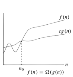
\(\Omega(g(n)) = \exists \, c > 0, n_{0} > 0\) \(s.t. \; 0 \leq cg(n) \leq f(n)\) \(\forall \, n \geq n _{0}\)

I will break this down into individual parts, then piece them together to arrive at the final equation. First, lets start with what's left of the equal sign.

\(\Omega(g(n))\)

\(\Omega\) is Big-Omega, which denotes the best-case time complexity or the lower-bounds for an algorithm. \(n\) is the input for the function \(g\). \(g\) is the function that describes the original algorithm. Next, lets look at

\(\exists \, c > 0, n_{0} > 0\)

The \(\exists \) denotes, "there exists". So the equation states that there exists two constants, \(c\) and \(n_{0}\) whose values both are greater than 0. \(c\) is simply a constant that accounts for operations that are not proportional to the input \(n\) for \(g\). \(n_{0}\) is a theoretical size for the input \(n\) wherein only after input size does \(\Omega\) actually maintain the lower-bound for \(g\). Remember, we do not give actual values for the variables, but leave them ambigious so that we have a lower-bound model to use for all algorithms.

\(0 \leq cg(n) \leq f(n)\)

\(0 \leq cg(n) \leq f(n)\) states that our lower bounds, \(g(n)\) times some constant \(c\) lies between \(0\) and our original function \(f(n)\). This makes sense as the lower-bound runtime for our algorithm cannot be less than 0 but also needs to be lower than or equal to the runtime of our original function. Otherwise it would not be much of a lower bound. Then there is \(0 \leq cg(n) \leq f(n)\). This means that \(cg(n)\) lies between \(0\) and \(f(n)\). In this instance, \(f(n)\) is the original asymptotic function, the one that is derived from the algorithm itself. \(cg(n)\) denotes the lower-bounds of our original asymptotic function times some constant \(c\). Thus, this is saying that the lower-bounds of the original asymptotic function for our algorithm lies at or below the original asymptotic function or at or above \(0\).

\(\exists \, c > 0, n_{0} > 0\) \(s.t. \; 0 \leq cg(n) \leq f(n)\)

Now, to put the last two parts together. This segment of the equation is saying that the lower-bounds of our original function \(g(n)\) times some constant \(c\) that is greater than 0, lies at or below the original function \(f(n)\) or at or above \(0\).

So looking at the final equation again:

\(\Omega(g(n)) = \exists \, c > 0, n_{0} > 0\) \(s.t. \; 0 \leq cg(n) \leq f(n)\) \(\forall \, n \geq n _{0}\)

This translates to, "There exists some contant \(c\) greater than \(0\) and some constant \(n_{0}\) such that \(cg(n)\) is greater than or equal to \(0\) and less than or equal to \(f(n)\) where all \(n\) are greater than or equal to \(n_{0}\)". From what we have learned we can say that this equation here says that there exists a constant \(c\) and \(n\), \(c\) being runtime constants, that are greater than \(0\) such that our lower-bound exists between \(0\) and the original asymptotic function.

Best-Case Time Complexity Graph