Quantum Support Vector Machine
My code for detecting credit card fraud using a Quantum Support Vector Machine: QuantumSVMFraudDetection
Introduction
Using quantum computing, the authors exploit quantum mechanics for the algorithmic complexity optimization of a support vector machine with high-dimensional feature space. Where the high-dimensional classical data is mapped non-linearly to Hilbert space and a hyperplane in quantum space is used to separate and label the data. By using the quantum state space as the feature space, the authors hope to obtain a quantum advantage.
Consider we have data from a training set \(T\) and a testing set \(S\), where \(T, S\) are subsets \(\Omega\subset\mathbb{R}^{d}\). For each training set, we assume the data is labeled by a true map \(m: T \cup S \rightarrow\left\{+1, -1\right\}\), which is not given to the algorithm. The algorithm is given training data, where the goal is for the algorithm to infer an approximate mappping \(\tilde{m}: T\rightarrow\{+1,-1\}\) for the data. After training, the algorithm is asked to apply the approximate mapping on a test set \(\tilde{m}: S\rightarrow\{+1,-1\}\). The approximate mapping needs to match the true map \(m(\vec{s})=\tilde{m}(\vec{s})\) with a high probability.
To use quantum state space as feature space a mapping is constructed such that the data is non-linearly mapped to a quantum state \(\Phi:\vec{x}\in\Omega\rightarrow |\Phi(\vec{x})\rangle\langle\Phi(\vec{x})|\). Where, \(|\Phi(\vec{x})\rangle\) is a part of complex vector space or Hilbert Space \(\mathcal{H}\) and \(\langle\Phi(\vec{x})|\) is the complex conjugate that is a dual correspondance. We can see that the non-linear mapping \(\Phi\) takes the classical data \(\vec{x}\in\Omega\subset\mathbb{R}^{d}\) or \(\vec{x}\in T\cup S\) and reperesents it in quantum state space \(|\Phi(\vec{x})\rangle\langle\Phi(\vec{x})|\). To continue, we will look at the procedure behind quantum mapping.
Quantum Feature Mapping
The authors suggest that in order to have an advantage over classical approaches, a map based on circuts that are clasically hard to simulate needs to be constructed, but where the circut is not too deep to test on during experimentation.
The authors provide a circut diagram that represents a unitary function for feature mapping \(n\)-qubits. The circut diagram is given as:
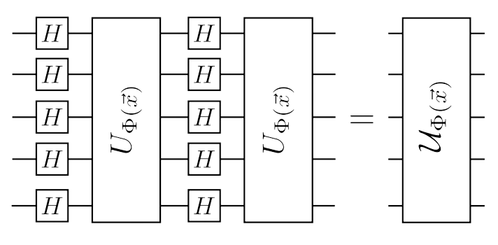
Image Source: \(^{[1]}\)
Note, we will examine more in depth the feature mapping unitary function later on.
Data Generation
First, we will define the map used for the artifical data. The data is generated of dimension \(n=d=2\) for a \(2\)-qubit system with the mapping \(\phi_{\{i\}}(\vec{x})=x_{i}\) and \(\phi_{\{1,2\}}(\vec{x})=(\pi-x_{1})(\pi-x_{2})\).
Next, we look at how the data is generated. For the data vector labels \(\vec{x}\in T\cup S \subset (0, 2\pi]^{2}\) the authors mention generating it using the parity function \(\mathbf{f}=Z_{1}Z_{2}\) and random unitary \(V\in SU(4)\).
Next, to label the data the authors describe the following mapping. Given \(\Delta=0.3\), if:
\(\langle\Phi(\vec{x})|V^{\dagger}\mathbf{f}V|\Phi(\vec{x})\rangle\geq\Delta\)
then \(m(\vec{x})=+1\). If:
\(\langle\Phi(\vec{x})|V^{\dagger}\mathbf{f}V|\Phi(\vec{x})\rangle\leq-\Delta\)
then \(m(\vec{x})=-1\).
Proposed SVM Classifiers
Quantum Variational Classification
In the this section, we will deconstruct and analyze individual components of the circut, unitary, and steps to better understand how this processes works. Then, in the following section, we will look at classifier optimization, testing the trained model, and analyze the authors experimental findings.
Procedure
The authors have provided a figure of the quantum variational classification QVC circut and it is shown below:
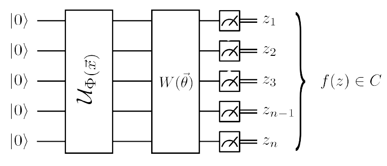
Image Source: \(^{[1]}\)
where \(C=\{+1,-1\}\) and the varitional unitary for QVC as a whole is defined as:
\(p_{y}(\vec{x})\)\(=\langle\Phi(\vec{x})|W^{\dagger}(\vec{\theta})M_{y}W(\vec{\theta})|\Phi(\vec{x})\rangle\)
The authors describe the procedure for the QVC in the following four sequential steps: feature map encoding, variational optimization, measurement, and then error probability. The training and classification phase consist of these four main parts and is what we will analyze in the following.
Feature Map Encoding
Recall that the circut looks like the following:
Image Source: \(^{[1]}\)
The data \(\vec{x}\in\Omega\) is mapped to a reference state \(|0\rangle^{n}\) using the feature map circut \(\mathcal{U}_{\Phi(\vec{x})}\). This feature map is an injective encoding of classical information \(\vec{x}\in\mathbb{R}^{d}\) to a quantum state \(|\Phi(\vec{x})\rangle\langle(\vec{x})\Phi|\) that is on a \(n\)-qubit register such that \(d=n\). A qubit is a two-level system of Hilbert space and can be represented as \(\mathcal{H}_{2}=\mathbb{C}^{2}\). To represent \(n\)-qubits we denote it as \(\mathcal{H}_{2}^{\otimes n}=\left(\mathbb{C}^2\right)^{\otimes n}\).
The offered feature mapping portrayed above is a family of feature maps, that the authors selected because they conjecture it is hard to estimate overlap \(|\langle\Phi(\vec{x}) \mid \Phi(\vec{y})\rangle|^2\) on a classical computer. The family of feature map circuits is defined as follows:
\(|\Phi(\vec{x})\rangle=U_{\Phi(\vec{x})} H^{\otimes n} U_{\Phi(\vec{x})} H^{\otimes n}|0\rangle^{\otimes n}\)
where \(H\) is a conventional Hadmard gate and \(U_{\Phi(\vec{x})}\) is defined as:
\(\exp\left(i\sum_{S\subseteq[n]}\phi_{S}(\vec{x})\prod_{i\in S}Z_{i}\right)\)
and is a diagonal gate in the Pauli Z-basis. For a single qubit, the unitary function \(U_{\Phi(x)}\) acts as a phase-gate \(Z_{x}\) of angle \(x\in\Omega\).
Feature mapping allows for \(2^{n}\) possible coefficents \(\phi_{S}\left(\vec{x}\right)\) for non-linear function of the inputed data \(\vec{x}\in\mathbb{R}^{n}\).
Variational Classification
A short depth quantum circut \(W(\vec{\theta})\) is applied to the feature state is a variational circut used for the optimization method. A depiction of this short depth quantum circut is given by the authors and shown in the figure below:
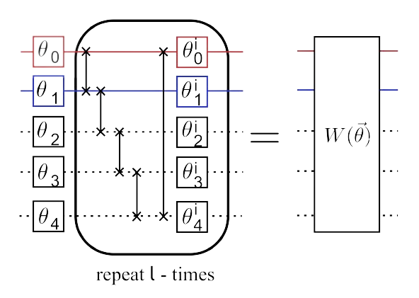
Image Source: \([1]\)
For this short depth quantum circut, the authors use an Ansatz variational unitary \(W(\vec{\theta})\), defined as:
\(U_{loc}^{(l)}(\theta_{l})U_{ent}...\)\(U_{loc}^{(2)}(\theta_{2})U_{ent}U_{loc}^{(1)}(\theta_{1})\)
Where, \(U_{loc}^{(l)}(\theta_{l})\) is full layers single qubit rotations given as:
\(U_{loc}^{(t)}(\theta_{t})=\bigotimes_{i=1}^{n}U(\theta_{i,t})\)
and \(U(\theta_{i,t})\in SU(2)\).
For the variational unitary, \(U_{ent}\) is an alternating layers of entangling gates and is defined as:
\(U_{ent}=\prod_{(i,j)\in E}\mathbf{CZ}(i,j)\)
Here, \(E\) is an edge in the circut defined vetice set \(\{v_{i}, v_{j}\}\in V\). \(\mathbf{CZ}\) is a controlled phase gate applied along the edges \((i,j)\in E\) which the authors state is present in the connectivity of the superconducting chip.
This variational circut is parametrized by \(\vec{\theta }\in\mathbb{R}^{2n(l+1)}\) and it is what is optimized during training as this is what classifies the data.
Measurement
Given that the problem is a two label classification \(y\in\{+1,-1\}\), the authors apply a binary measurment \(\{M_{y}\}\) to the state \(W(\vec{\theta})\mathcal{U}_{\Phi(\vec{x})}|0\rangle^{n}\).
The authors describe the binary measurment in the following way. The measurment is in the \(Z\)-basis, outputs the bit-string \(z\in\{0,1\}^{n}\), where the bit-string is then passed to the boolean function \(f:\{0,1\}^{n}\rightarrow\{+1,-1\}\). The binary measurment is defined as \(M_{y}=2^{-1}(\mathbb{1}+y\mathbf{f})\), where \(\mathbf{f}=\sum_{z\in\{0,1\}^n}f(z)|z\rangle\langle z|\).
From this third step, the probability for the outcome \(y\) is obtained. This probability \(p_{y}(\vec{x})\) is defined as:
\(p_{y}(\vec{x})\)=\(\langle\Phi(\vec{x})|W^{\dagger}(\vec{\theta})M_{y}W(\vec{\theta})|\Phi(\vec{x})\rangle\)
Where the probability for measuring either label \(y\in\{+1,-1\}\), denoted as \(p_y\), is defined as:
\(\frac{1}{2}\left(1+y\left\langle\Phi(\vec{x})\left|W^{\dagger}(\theta)\right.\right.\right.\)\(\left.\left.\left.\mathbf{f} W(\theta)\right| \Phi(\vec{x})\right\rangle\right)\)
Since the expected value of the measured observable is \(\operatorname{tr}\left[|\Phi(\vec{x})\rangle\langle\Phi(\vec{x})| W^{\dagger}(\theta, \varphi)\right.\)\(\left.\mathbf{f} W(\theta, \varphi)\right]\), it can be expressed in terms of the inner product:
\(\frac{1}{2^n} \sum_\alpha w_\alpha(\theta) \Phi_\alpha(\vec{x})\)
Next, we need to incorporate assigning the label \(y\in\{+1,-1\}\) over the label \(-y\) with a given fixed basis \(b\in[-1,+1]\). In this case, it must be that \(p_{-y}-yb<\ p_{y}\). Subsituting the probability for measuring either label \(y\in\{+1,-1\}\) in to the inner product of the measured observable, we obtain the value for \(\tilde{m}(\vec{x})\) as:
\(\operatorname{sign}\left(\frac{1}{2^n} \sum_\alpha w_\alpha(\theta) \Phi_\alpha(\vec{x})+b\right)\)
For the final decision ruling of \(y\), \(R\) repeated measurment shots are preformed, yielding the empircal distribution \(\hat{p}(\vec{x})\), where if \(\hat{p}_{-y}(\vec{x}-yb)>\hat{p}_{y}(\vec{x})\) the label assigned is \(\tilde{m}(\vec{x})=y\). The authors introduced a bias parameter \(b\in[-1,1]\) that can also be optimized during training.
The authors mention that the feature map circut \(\mathcal{U}_{\Phi(\vec{x})}\) and the boolean function \(f\) are fixed choices. The parameters that are being optimized during training are \((\vec{\theta},b)\) and in order to be optimized, a cost-function is need to be defined. To do so, we need to define an error probability first, which is what we will look at in the next section.
Error Probability
In order to find the empirical risk \(R_{emp}(\vec{\theta})\) of the empirical distribution \(\hat{p}(\vec{x})\) we define the error probability of assigning the incorrect labels averaged over the samples in the training set \(T\). The authors give the definition:
\(R_{emp}(\vec{\theta})\) \(=\) \(\frac{1}{|T|}\sum_{\vec{x}\in T}Pr(\tilde{m}(\vec{x})\neq m(\vec{x}))\)
that defines this error probability. For our binary classification problem, the error probability of assigning the wrong label to some given data can be clacilated using the binomial cimulative density function CDF for the empircal distribution \(\hat{p}(\vec{x})\). For a large number of samples or shots \(R\gg 1\) the CDF is approximated by a sigmoid function \(\operatorname{sig}(x)=(1+e^{-x})^{-1}\). The probability for label \(m(\vec{x}=y)\) being assigned incorrectly can be approximated by:
\(Pr(\tilde{m}(\vec{x})\neq m(\vec{x}))\)
\(\approx\operatorname{sig}\left(\frac{\sqrt{R}\left(\frac{1}{2}-\left(\hat{p}_y(\vec{x})-\frac{y
b}{2}\right)\right)}{\sqrt{2\left(1-\hat{p}_y(\vec{x})\right)
\hat{p}_y(\vec{x})}}\right)\)
Classifier Optimization and Testing Results
The first step is to train the classifier and optimize it. The authors found that they found Spall's SPSA stochastic gradient descent algorithm performs the best in the inherent noisy experimental setting of quantum computing. They mentioned after the parameters converged onto \(\big(\vec{\Theta^{*}},b^{*}\big)\). The second step is then to classify data and assign them labels according to the decision rule given by \(\tilde{m}(\vec{s})\), where the binary measurement is obtained from the parity function \(\mathbf{f}=Z_1 Z_2\), and ensure that for the testing data, \(m(\vec{s})=\tilde{m}(\vec{s})\) with high probability for the given data set \(\vec{s}\in S\).
The authors note that what is obeserved for the empirical risk, or cost value used for the optimizer, is that it converges to a lower depth when the number of layers in the short depth quantum circuit for optimization is \(l=4\) than \(l=0\). Interesting enough, error mitigation does not appreciably improve the empirical risk results when depth is at \(0\), however, does substantially help for larger depths. An important note, is that although \(\operatorname{Pr}(\tilde{m}(\vec{x}) \neq m(\vec{x}))\) includes the number of shots \(R\) taken in its calculation, during experimentation the authors fixed \(R=200\). The authors state the reason for doing this, even though \(R=2000\) in actual experiment, was to avoid gradient problems.
To continue, after training, comes testing. The yielded trained set of parameters \(\big(\vec{\theta}^{*},b^*=0\big)\) where used to classify 20 different test sets randomly drawn each time per data set. After analyzing the results, the authors an increasing classification success with increasing circut depth \(l\). Noting, that the success rate very nearl reaches \(100\)% for circut depths larger than \(1\) and remains up to depth \(4\), despite decoherence associated with \(8\) CNOT gates during training and classification circuts.
Quantum Variational Classification Analysis
An important aspect of SVM's, is the classification of the data, which is done here based off of the decision rule \(p_y(\vec{x})>p_{-y}(\vec{x})-y b\). This decision rule \(\tilde{m}(\vec{x})\) can can be restated as \(\operatorname{sign} \big( \langle\Phi(\vec{x}) |W^{\dagger}(\vec{\theta})\)\( \mathbf{f} W(\vec{\theta}) | \Phi(\vec{x}) \rangle+b \big)\). The step that structures the data in such a way for classification, is the variational circut \(W\), which seperates the data using hyperplane \(\vec{w}\) in quantum state space. A feature map of a single qubit, along with the seperating hyperplane \(\vec{w}\) and the invterval of binary labels \(\Omega=(0,2\pi]\) for the classical data, is given by the authors below.
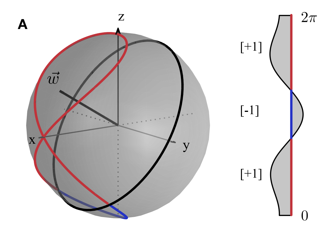
Image Source: \([1]\)
We start by decomposing the quantum variational circut. First, we look to define the properties for our group of matrices used. For us, we need a group that has an orthogonal, hermatian, matrix basis \(\left\{P_\alpha\right\} \subset \mathbb{C}^{2^n \times 2^n}\). Such that \(\alpha=1,...,4^{n}\) with \(\operatorname{tr}\left[P_\alpha^{\dagger} P_\beta\right]=2^n \delta_{\alpha, \beta}\). A group of matrices adhereing to this criteria is the Pauli-group on \(n\)-qubits. Next, we expand the quantum state and the measurment in our choosen matrix basis.
The expanded quantum state, or expectation value, can be expressed in terms of \(|\Phi(\vec{x})\rangle\langle\Phi(\vec{x})|\) \(\rightarrow\) \(\Phi_\alpha(\vec{x})=\left\langle\Phi(\vec{x})\left|P_\alpha\right| \Phi(\vec{x})\right\rangle\). The decision rule expressed in our choosen matrix basis as \(w_\alpha(\vec{\theta})\) can be defined as \(W^{\dagger}(\vec{\theta}) \mathbf{f} W(\vec{\theta})\) \(\rightarrow\) \(\operatorname{tr}\left[W^{\dagger}(\vec{\theta}) \mathbf{f} W(\vec{\theta}) P_\alpha\right]\). Lastly, any classification rule or mapping \(\tilde{m}(x)\) from a variational unitary can be restated in the SVM form:
\(\operatorname{sign}\left(2^{-n} \sum_\alpha w_\alpha(\vec{\theta}) \Phi_\alpha(\vec{x})+b\right)\)
What we can see is that the behavior of the classifier is dependent on the larger term \(\omega_{\alpha}\), so by improving this term, this constraining term is lifted from the variational circut. The authors note as well that the optimal value for \(\omega_{\alpha}\) can alternatively be found through implementing kernel methods and the Wolfe dual approach of the SVM. The important idea we can gain from decomposing of variational circut, is that we can think of the feature space as the quantum state space that has feature vectors \(|\Phi(\vec{x})\rangle\langle\Phi(\vec{x})|\) and inner products \(K(\vec{x}, \vec{z})=|\langle\Phi(\vec{x}) \mid \Phi(\vec{z})\rangle|^2\).
With this more clear image of how feature space is being represented as quantum state space, we can see that the direct use of Hilbert space for this can lead to conceptual errors. Such that, a vector in Hilbert space \(|\Phi(\vec{x})\rangle \in \mathcal{H}\) is only defined up to a global phase physically.
What was seen was that a quantum advantage is mainly obtained from feature maps that have a classicaly hard to estimate kernel.
Quantum Kernel Estimation
Procedure
Unlike, in a variational quantum circut to generate a seperating hyperplane for the high-dimesnional feature space, Quantum Kernel Estimation a classical SVM classification instead. Meaning, this type of classification does not make a direct use of Hilbert space, allowing for it to side step the inherent conceptual errors of that quantum variational classification feature map representation.
To continue.
Quantum Feature Mapping Implementations for Support Vector Machines
A feature map can be denoted as \(\Phi: \Omega \subset \mathbb{R}^d \rightarrow \mathcal{S}\left(\mathcal{H}_2^{\otimes n}\right)\) such that \(\Phi: \vec{x} \mapsto|\Phi(\vec{x})\rangle\langle\Phi(\vec{x})|\). The map acting on the data input is a unitary circut family \(\mathcal{U}_{\Phi(\vec{x})}\) applied to \(|0\rangle^n\). The result can be denoted as \(|\Phi(\vec{x})\rangle=\mathcal{U}_{\Phi(\vec{x})}|0\rangle^n\), such that the state in the feature space is linearly independent.
Let's analyze a feature map corresponding to a product state. First, assume that a feature map is comprised of single qubit rotations \(U(\varphi) \in \mathrm{SU}(2)\) aranged in a quantum circuit. These angles correspond to a non-linear function \(\varphi: \vec{x} \rightarrow(0,2 \pi]^2 \times[0, \pi]\) mapped to the space of Euler angles. This means that the feature mapping action for an individual qubit is:
\(\vec{x} \mapsto\left|\phi_i(\vec{x})\right\rangle=U\left(\varphi_i(\vec{x})\right)|0\rangle\)
and the feature mapping action for the full qubit state is:
\(\Phi: \vec{x} \mapsto|\Phi(\vec{x})\rangle\left\langle\Phi(\vec{x})|\right.\)\(\left.=\bigotimes_{i=1}^n| \phi_i(x)\right\rangle\left\langle\phi_i(x)\right|\)
Stoudenmire and Schwab using tensor networks is an example of unitary implementation of feature mapping of classical classifiers. In this implementation, each qubit encodes a single component \(x_{i}\) of \(\vec{x}\in[0,1]^{n}\), thus, using \(n\) qubits. The prepared state of this full qubit feature mapping encoding when expanded to the Pauli-matrix basis:
\(\bigotimes_{i=1}^n\left|\phi_i(x)\right\rangle\left\langle\phi_i(x)\right|\) \(=\) \(\frac{1}{2^n} \bigotimes_{j=1}^n\left(\sum_{\alpha_j} \Phi_j^{\alpha_j}\left(\theta_j(\vec{x})\right) P_{\alpha_j}\right)\)
Such that, with respect to the Pauli-matrix basis, \(\Phi_i^\alpha\left(\theta_i(\vec{x})\right)\) \(=\) \(\left\langle\phi_i(x)\left|P_{\alpha_i}\right| \phi_i(x)\right\rangle\) for every \(i=1\dots,n\) and where \(P_{\alpha_i} \in\left\{\mathbb{1}, X_i, Z_i, Y_i\right\}\).
To continue.