Quantum Computing Theory

Introduction

Quantum Computing Theory is a field of computer science that uses the principles of quantum mechanics, mathematics, and computer science. By borrowing concepts from each field scientists can rigorously define both a broad and narrow theoretical model of a quantum computer and later apply it to the real world. Quantum computers utilize the result of manipulating subatomic particles and abstract theoretical circuits are just a few of the fundamental concepts in quantum computing theory we will look at in this article.

One Qubit

Qubit

A qubit, short for quantum bit, is a two-level quantum system and is a part of two-dimensional Hilbert space \(H_{2}\), where Hilbert space \(H\) is a nondenumerable infinite complex vector space. The two-dimensional complex vector space \(H_{2}\) comes with a fixed orthonormal basis states \(B=\left\{|0\rangle,|1\rangle\right\}\) when the base measurement is in the \(Z\) basis. States \(|0\rangle\) and \(|1\rangle\) are the basis states, denoted with Dirac notation.

The states of the quantum system or qubit can be denoted as a vector like:

\(a|0\rangle + b|1\rangle\)

This vector has a unit length of \(1\), so \(|a|^{2} + |b|^{2}=1\). Here, the eigenvalues \(|a|^{2}\) and \(|b|^{2}\) are the probabilities of the system being in their respective eigenvectors. This means that the quantum system is measured, it will give a state \(0\) or \(1\) in this two-level quantum system with respective probabilities. We will go more in-depth into probabilities here soon.

First, however, we will look at formal definition of the inner dot product of some given some qubit \(\theta\). For \(|\theta\rangle\) the unit length is equivalant to its inner product. Where, for ket \(|\theta\rangle\) and bra \(\langle\theta|=(a^{*}b^{*})\), \(a,b\) are both complex numbers and both have two real numbers. The inner dot product is \(|\theta\rangle|\theta^{*\intercal}\rangle=|\theta\rangle|\theta^{\dagger}\rangle\), formulated as:

\(\langle\theta|\theta\rangle=(a^{*}b^{*})\begin{pmatrix}a\\b\end{pmatrix}=|a|^{2}+|b|^{2}=1\)

For some quantum state for the qubit \(\psi\) can be defined as:

\(|\psi\rangle=\begin{pmatrix}\cos(\theta)\\ \sin(\theta)\end{pmatrix}\)

\(=\langle v|\psi\rangle|v\rangle+\langle h|\psi\rangle|h\rangle\)

Where, squaring our projections, \(\langle v|\psi\rangle\) and \(\langle h|\psi\rangle\), onto axis an axis gives us our respective probabilites for \(|v\rangle\) and \(|h\rangle\) respectfully.

An example of a qubit is the spin of an electron. The two levels of this qubit are spin up or spin down. What differs from a classical system is that quantum mechanics allows for the qubit to be in a coherent superposition of both states simultaneously.

Measuring a qubit in a basis gives a projective measurement of a qubit of state \(\phi\) in its computational basis can be expressed as a linear combination of state vectors, such as:

\(|\psi\rangle=a|0\rangle+b|1\rangle\)

When the qubit is measured in a basis, collapses the qubit to either the quantum state \(|0\rangle\) or \(|1\rangle\) given by the respective norm-square of the probability amplitudes \(a\) and \(b\), or \(a^{2}\) and \(b^{2}\).

Bloch Sphere

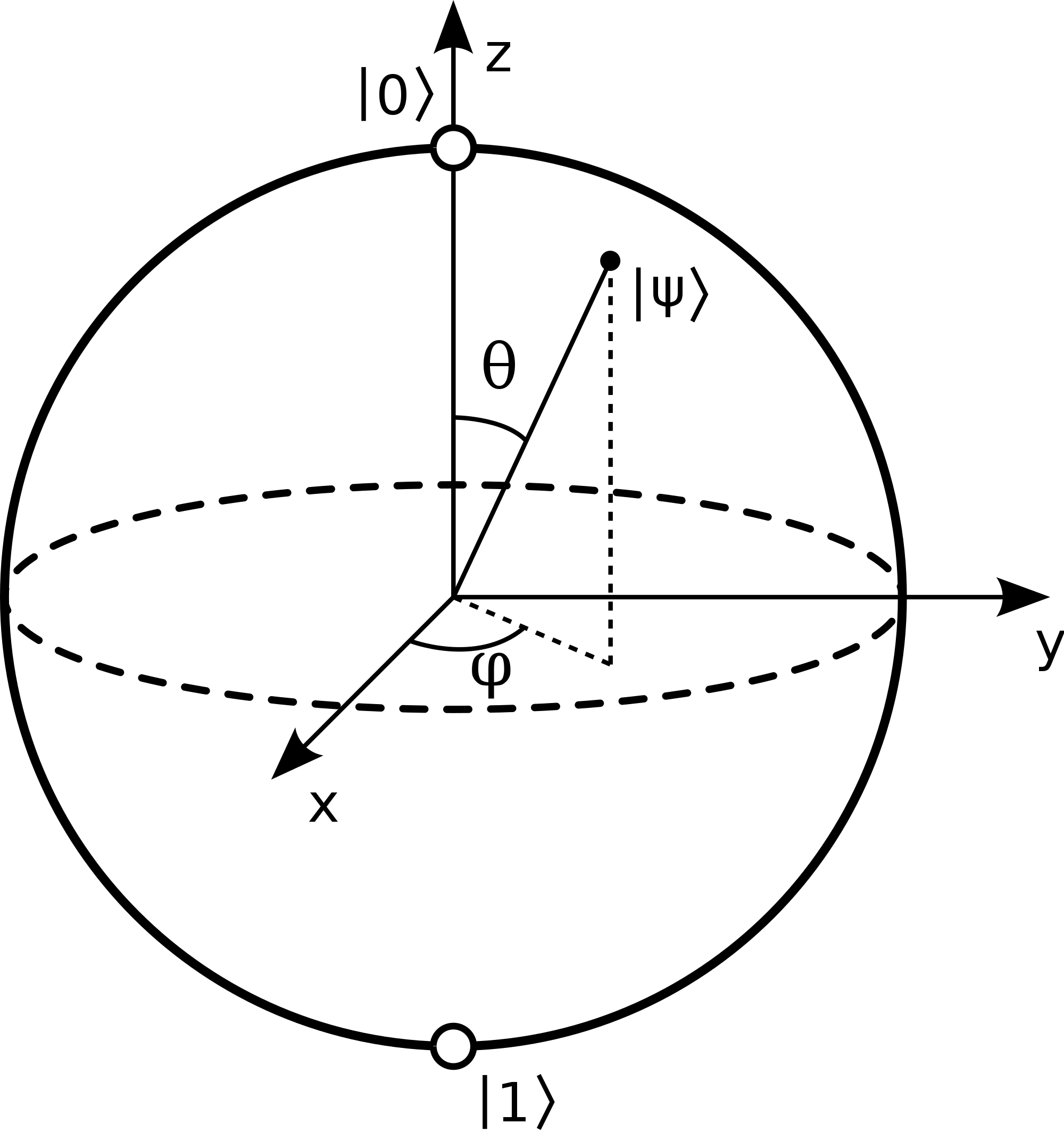
We can use a bloch ball or sphere to help us visualize sping down \(0\) and spin up \(1\) of a single qubit. The bloch spehere has a radius of 1, meaning that \(|0\rangle\) corresponds to \((x,y,z)\) point \((x,y,1)\) and \(|1\rangle\) corresponds to \((x,y,z)\) point \((x,y,-1)\). Where our \(z\) value shows a spin up or sping down.

Superposition

In classical computing, states \(0\) and \(1\) would be the only states that exist for the bit. However, in quantum mechanics a qubit can be both in the state of \(|0\rangle\) and \(|1\rangle\). This is what gives quantum computers more processing power, as a single qubit can be in more states and therefore represent more information than a single classical bit.

This means that the qubit can have an \(80\)% of being in state \(|0\rangle\) and \(20\)% of being in state \(|1\rangle\), or \(75\)% of being in state \(|0\rangle\) and \(25\)% of being in state \(|1\rangle\). Unlike a classical bit where there is either a \(100\)% of the classical bit being in state \(0\) and \(0\)% of being a \(1\) or a \(0\)% of the classical bit being a \(0\) and \(100\)% of being a \(1\). To allow for the qubit to be in superposition, we need to levearage Hilbert Space. Again, Hilbert space is represented using complex vector space. We use complex vector space, because it is the easiest way for the math to work.

Let's represent this qubit in superposition as a vector using dirac notation. For the qubit have, for example, a \(50\)% of being in state \(|0\rangle\) and \(50\)% of being in state \(|1\rangle\), the vector should look like:

\(\frac{1}{\sqrt{2}}(|0\rangle+|1\rangle)\)

The coefficent for \(0\) and \(1\) are both \(\frac{1}{\sqrt{2}}\) and therefore equal parts \(0\) and \(1\).

Pauli Matrices

Pauli matrices have a core importance in quantum physics, and when combined with an identity matrix, pauli matrices form a basis for all single quantum gates. Pauli matrices are defined as:

\(\sigma_{x}=\begin{pmatrix} 0&1 \\ 1&0 \end{pmatrix}\),

\(\sigma_{y}=\begin{pmatrix} 0&-i \\ i&0 \end{pmatrix}\),

\(\sigma_{z}=\begin{pmatrix} 1&0 \\ 0&-1 \end{pmatrix}\)

\(\sigma_{x}\) is usally refered to as the NOT gate and can be written as \(X\). The NOT gate inverts \(|0\rangle\) and \(|1\rangle\) and \(\sigma_{y}\), \(\sigma_{z}\) are phase shifting gates.

To continue.

Multiple Qubits

Quantum Registers

A system that contains more than one qubit is represented in a quantum register. A system with two qubits is represented using a four-dimensional Hilbert space \(H_{4} = H_{2} \otimes H_{2}\). The orthonormal basis is \(\left\{|0\rangle |0\rangle, |0\rangle |1\rangle, |1\rangle |0\rangle, |1\rangle |1\rangle\ \right\}\). \(|0\rangle |0\rangle\) can be more succinctly written as \(|00\rangle\). The same is true for \(|0\rangle |1\rangle = |01\rangle\), etc. A state of this two-qubit system, a part from four-dimensional Hilbert space is a unit-length vector:

\(c_{0}|00\rangle + c_{1}|01\rangle + c_{2}|10\rangle + c_{3}|11\rangle\)

Again, as it is with a single qubit, it is required that \(|c_{0}|^{2} + |c_{1}|^{2} + |c_{2}|^{2} + |c_{3}|^{2} = 1\).

Observations of this two-qubit system will give \(00\), \(01\), \(10\), and \(11\) with the outcomes \(|c_{0}|^2, |c_{1}|^2, |c_{2}|^2, |c_{3}|^2\), respectively. If we want to observe one of the qubits, then the standard rules of probabilities apply.

It is important to note that the tensor product of these vectors does not commute. Meaning, that \(|0\rangle|1\rangle \neq |1\rangle|0\rangle\). Linear ordering is used to address the qubits individually.

Quantum Entanglement

Maximally Entangled Bell States

Bell states or Einstein, Podolski and Rosen pairs are the maximally entangled quantum states of a qubit system such that a quantum mechanical system is composed of two interacting two-level subsystems. The 4 types of maximially entangled Bell states can be defined as:

\(|\Phi^{+}\rangle = \frac{|00\rangle+|11\rangle}{\sqrt{2}}\)

\(|\Phi^{-}\rangle = \frac{|00\rangle-|11\rangle}{\sqrt{2}}\)

\(|\Psi^{+}\rangle = \frac{|01\rangle+|10\rangle}{\sqrt{2}}\)

\(|\Psi^{-}\rangle = \frac{|01\rangle-|10\rangle}{\sqrt{2}}\)

Measurments

Bases Measurments

The orthagonal basis states for \(Z\), \(X\), and \(Y\), are as follows:

\(Z=\{|0\rangle,|1\rangle\}\)
\(X=\{|-\rangle,|+\rangle\}\)
\(Y=\{|i\rangle,|-i\rangle\}\)

X Bases Measurment

To measure from the \(Z\) basis to the \(X\) bases, we need to apply a Hadmard gate to the state, allowing for the state to be halfway:

\(H|0\rangle=|+\rangle=\begin{pmatrix}\frac{1}{\sqrt{2}}\\ \frac{1}{\sqrt{2}}\end{pmatrix}\) \(=\frac{1}{\sqrt{2}}(|0\rangle+|1\rangle)\)

\(H|1\rangle=|-\rangle=\begin{pmatrix}\frac{1}{\sqrt{2}}\\ -\frac{1}{\sqrt{2}}\end{pmatrix}\) \(=\frac{1}{\sqrt{2}}(|0\rangle-|1\rangle)\)

Y Bases Measurment

Then to measure from the \(Z\) basis to the \(Y\) bases, we need to apply a Hadmard gate to the state, allowing for the state to be halfway we need to apply \(S^{*\intercal}=S^{\dagger}\):

\(\frac{1}{\sqrt{2}}\begin{pmatrix}1 & -i\\1 & i \end{pmatrix}^{\dagger}=\frac{1}{\sqrt{2}}\begin{pmatrix}1 & 1\\i & -i \end{pmatrix}\)

Z Bases Measurment

No transformations needed, since we measure in the "normal" bases.

Operators

Unitary Operator

All quantum gates are unitary, which we will define in the following. Let us use the basis measurment of \(Z\) with the coordinate representation \(|0\rangle = \begin{bmatrix} 1\\ 0 \end{bmatrix}\) and \(|1\rangle = \begin{bmatrix} 0\\ 1 \end{bmatrix}\).

An operation on a qubit, called an unary quantum gate, is a unitary mapping \(U: H_{2} \rightarrow H_{2}\) with the following defining linear operation:

An important aspect of all quantum gates is that they are unitary. Meaning, that for some given matrix operation \(U\), defined as:

\(\begin{pmatrix} a & b \\ c & d \end{pmatrix}\)

it is neccesary that this matrix is unitary in order to be a valid quatnum gate. So, for some matrix or operator \(U\) to be unitary and valid, the following equivalency must be true:

\(UU^{\dagger}=I\)

where \(U^{\dagger}\) represents the conjugate transpose and \(I\) is the identity matrix.

Another important qualtiy of an unitary matrix is:

\(U^{\dagger}=U^{-1}\)

Represented as matrices, we get:

\(\begin{pmatrix} a & b \\ c & d \end{pmatrix} \begin{pmatrix} a^* & b^* \\ c^* & d^* \end{pmatrix} = \begin{pmatrix} 1 & 0 \\ 0 & 1 \end{pmatrix}\)

Written in vector form, the conjugate transpose of \(U\) is denoted as \(U^{\dagger}\) and can be wrriten as:

\(\begin{pmatrix}a\\ d\end{pmatrix}^{\dagger}=\left(a^{*}d^{*}\right)\)

where the notation \(a^{*}\) stands for the complex conjugate of the complex number \(a\). The complex conjugate of a complex number is the number with an equal real part and an imaginary part equal in magnitude, but opposite in sign of the complex number.

The mapping of for unary quantum operator, when represented in a quantum circut, can be a quantum gate. Where the output of the quantum gate must have the same dimensionality as its input. So, \(U: H_{n} \rightarrow H_{n}\), where \(n\) is the number of dimensions of \(H\).

Hermitian Operator

A unitary operator is Hermitian if:

\(U^{\dagger}=U\), where \(U^{\dagger}\) is the conjugate transpose of the matrix \(U\).
\(U^{2}=I\), where \(I\) is an identity matrix.

A Hermatian matrix is a special case of a unitary matrix, where all Hermitian operators or unitary operators, but not all unitary operators, are Hermitian.

Natural Operator

An Hermitian operator is Natural if:

\(U^{\dagger}U=UU^{\dagger}\), where \(U^{\dagger}\) is the conjugate transpose of \(U\).
the operator has spectural decomposition, where \(U\) can be decomposed as:
\(U=\sum_{i}\lambda_{i}|\lambda_{i}\rangle\langle\lambda_{i}|\)

Quantum Algorithms

Quantum Parallelism

Suppose we want to evaluate a function \(f(x)\), where the function \(f\) expresses some computation or algorithm. A use case for quantum parallelism is to evaluate \(f(x)\) with many different values for the output of the computation or algorithm on the input \(x\) simultaneously. In essence, we can evaluate many different values of \(x\) on \(f\) in parallel by exploiting quantum effects. This quantum effect exploit feature is fundamental in many quantum algorithms. To continue, we will look at how quantum parallelism works.

Consider the one-bit domain and range function \(f(x):\{0,1\}\rightarrow\{0,1\}\). To compute this function \(f\) on a quantum computer, we will use a two-qubit quantum computer with the starting state \(|x,y\rangle\). The transformation on the domain or 'data' register to the range or 'target' register of this initial two qubit state is described by the following unitary function:

\(U_{f}:|x,y\rangle\rightarrow|x,y\oplus f(x)\rangle\)

where the \(\oplus\) represents addition modulo 2 and \(x=q_{0}, y=q_{1}\). When \(\oplus\) acts on \(y\), and its value is \(0\) then the value of the second qubit in the 'target' register is the value \(f(x)\), given whatever function \(f\) represents. The functions effect on \(x\) is arbritrary for now.

The final collapsed state \(|\psi\rangle\) is an element of the set of final states or 'target' register \(|x,y\oplus f(x)\rangle\), which again is given by the unitary transformation \(U_{f}\) on the start state \(|x,y\rangle\).

Given the input \(q_{0}=x=|0\rangle\), we will apply the Hadmard gate \(H\) to \(x\), such that now:

\(x=\frac{|0\rangle+|1\rangle}{\sqrt{2}},y=|0\rangle\)

where the resulting state is:

\(\frac{|0 f(0)\rangle+|1 f(1)\rangle}{\sqrt{2}}\)

which the resulting new state is not apart of the starting computational basis \(\{0,1\}\). Next, the unitary function or blackbox computation/algorithm \(U_{f}\) can be applied to the current 'data' register. The resulting mapping of the unitary function \(U_{f}\) is:

\(U_{f}\left(\frac{|0\rangle+|1\rangle}{\sqrt{2}},|0\rangle\right)=\frac{|0, f(0)\rangle+|1, f(1)\rangle}{\sqrt{2}}\)

\(=\frac{1}{\sqrt{2}}(|0,f(0)\rangle+|1,f(1)\rangle)\)

\(=.5|0,f(0)\rangle+.5|1,f(1)\rangle\)

Meaning that the final resulting state for a two-qubit quantum computer has a \(50\)% chance of being \(|0,f(0)\rangle\) and \(50\)% of being \(.5|1,f(1)\rangle\). Given in the same form as the range for \(U_{f}\) given above:

\(|x,y'\rangle\), where \(y'=y\oplus f(x)\)

All of this means that the information given by the mapping for \(f(0)\) and \(f(1)\) was simultaneously evaluated by applying superposition and the unitary function on the starting 'data' register. Thus, \(f(x)\) has been computed for two values of \(x\) in parellel. The resulting set of all possible states computed in parallel is given by the resulting 'target' register is given by quantum exploitation and aptly named 'quantum parallelism'. Thus, a single \(f(x)\) circuit can be used to evaluate the result for \(n\) values of \(x\) simultaneously.

Deutsch's Algorithm

Consider a two-qubit system such that \(q_{0}=x=|0\rangle,q_{1}=y=|0\rangle\). Now, let's apply the NOT gate to \(y\), giving the what will be the start state \(|\psi_{0}\rangle=|01\rangle\). Next, we will apply a Hadmard gates to \(x\) and \(y\) individually, yielding the state:

\(|\psi_{1}\rangle=\left[\frac{|0\rangle+|1\rangle}{\sqrt{2}}\right]\left[\frac{|0\rangle-|1\rangle}{\sqrt{2}}\right]\)

where for state \(|\psi_{1}\rangle\):

\(x=\frac{|0\rangle+|1\rangle}{\sqrt{2}}\)
\(y=\frac{|0\rangle-|1\rangle}{\sqrt{2}}\)

Applying some arbritrary unitary function \(U_{f}\) on \(|xy\rangle\) or \(|\psi_{1}\rangle\) gives:

\(|\psi_{2}\rangle=\left(-1\right)^{f(x)}\left[\frac{|0\rangle-|1\rangle}{\sqrt{2}}\right]\left[\frac{|0\rangle-|1\rangle}{\sqrt{2}}\right]\)

From this, we can then say that if \(f(0)=f(1)\):

\(|\psi_{2}\rangle=\left[\frac{|0\rangle+|1\rangle}{\sqrt{2}}\right]\left[\frac{|0\rangle-|1\rangle}{\sqrt{2}}\right]\)

or if \(f(0)\neq f(1)\):

\(|\psi_{2}\rangle=\left[\frac{|0\rangle-|1\rangle}{\sqrt{2}}\right]\left[\frac{|0\rangle-|1\rangle}{\sqrt{2}}\right]\)

Next step in Deutsch's algorithm is to apply a Hamdmard gate \(H\) to \(x\). If \(f(0)=f(1)\), the resulting state is:

\(|\psi_{3}\rangle=\pm|0\rangle\left[\frac{|0\rangle-|1\rangle}{\sqrt{2}}\right]\)

or if \(f(0)\neq f(1)\)

\(|\psi_{3}\rangle=\pm|1\rangle\left[\frac{|0\rangle-|1\rangle}{\sqrt{2}}\right]\)

This can then be written more succenctly as:

\(|\psi_{3}\rangle=\pm f(0) \oplus f(1) \left[\frac{|0\rangle-|1\rangle}{\sqrt{2}}\right]\)

Thus, \(f(0)\) interfers with \(f(1)\) when we simultaneously evalute \(f(x)\) with quantum parallelism.

Grovers Search Algorithm

The authors describe the process for Grovers Search Algorithm in the following sequential two main steps: Hadmard transformation and Grover iteration or Grover operator \(G\).

Hadmard Transformation

The Hadmard transform puts the qubits of the quantum computer into equal superposition states, defined as:

\(|s\rangle=|+\rangle^{\otimes n}=\frac{1}{\sqrt{N}} \sum_{x \in\{0,1\}^n}|x\rangle\)

Grover Operation

Grovers search algorithm implements a repeated quantum subroutine called Grover iteration or operator, denoted as \(G\). This quantum iteration can be broken up in four steps:

Apply oracle \(O\)
Apply Hadmard transform \(H^{\otimes{n}}\)
Apply conditional phase shift on quantum register, such that every quantum basis state except \(|r\rangle\) is phased shifted \(-1\). Meaning that for unitary:

\(\begin{aligned} U_f|s\rangle & =(-1)^1 \sin \theta|w\rangle \\ & +(-1)^0 \cos \theta|r\rangle \\ & =-\sin \theta|w\rangle+\cos \theta|r\rangle \end{aligned}\)

This phase kicks \(|w\rangle\) only. Then, reflect the state around \(|s\rangle\) using gate \(R_{s}\), such that moving our state towards \(|w\rangle\).

Lastly, apply the Hadmard transform \(H^{\otimes{n}}\)

Where combined steps of 2, 3, 4, or Grovers iteration without the oracle step can be written as:

\(H^{\otimes n}(2|0\rangle\langle 0|-I) H^{\otimes n}=2|\psi\rangle\langle\psi|-I\)

where \(|\psi\rangle\) is equaly eighted superposition of states \(\frac{1}{N^{1 / 2}} \sum_{x=0}^{N-1}|w\rangle\). Thus, including the oracle step now, Grovers iteration \(G\) as a whole can be written, more generically for a given quantum state \(\psi\) as \(G=(2|\psi\rangle\langle\psi|-I) O\). The circut is given as:

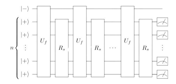
Image Source: \([1]\)

To continue.

Quantum Computational Theory

Quantum Automata Theory

Quantum Turing Machine

A Quantum Turing Machine QTM can be expressed similarly to a traditional Turing Machine TM with all components reformulated canonically except for the transition function \(\delta\). Below, is the formal definition of a QTM.

Quantum Turing Machine is a 7-tuple:

\((Q, \Sigma, \Gamma, \delta, q_{0}, q_{accept}, q_{reject})\)

where \(Q, \Sigma, \Gamma\) are all finite sets and:

\(Q\) is a set of states
\(\Sigma\) is an alphabet not containing the blank symbol \(\sqcup\)
\(\Gamma\) is the tape alphabet, where \(\sqcup \in \Gamma\) and \(\Sigma \subseteq \Gamma\). The tape is assumed to be two-way infinite, with squares indexed by the set of integers \(\mathbb{Z}\)
\(\delta\) is a transition function described as \(\delta : Q \times \Gamma \rightarrow \mathbb{C}^{Q \times \Gamma \times \left\{-1, +1\right\}}\)
\(q_{0} \in Q\) is the initial state
\(q_{accept} \in Q\) is the accept state
\(q_{reject} \in Q\) is the reject state, where \(q_{reject} \neq q_{accept}\)

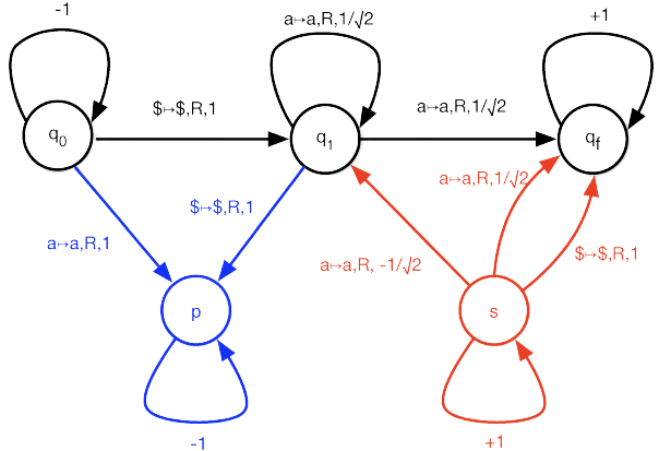
Image Source: https://www.mdpi.com/applsci/applsci-10-05551/article_deploy/html/images/applsci-10-05551-g004.png

Quantum Networks

Superdense Coding and Quantum Teleportation

Superdense Coding

Given Alice wants to send classical information to Bob, quantum entanglement \(n\) qubits can store \(2n\) qubits total of information. Say Alice needs to send one qubit of infromation, they can do so but needs Bob to already share a second qubit. So, given that Alice and Bob already share a pair of entangled qubits in state \(|\Phi^{+}\rangle\), defined as:

(Alice) -- \(\frac{1}{\sqrt{2}}(|00\rangle+|11\rangle)\) -- (Bob)

If Alice wants to send:

\(00\): Alice does nothing to their qubit, so the qubit is still in state:

\(|\Phi^{+}\rangle=\frac{1}{\sqrt{2}}(|00\rangle+|11\rangle)\)

\(01\): Alice applies \(X\) gate to their qubit, transforming \(|\Phi^{+}\rangle\) to:

\(|\Psi^{+}\rangle=\frac{1}{\sqrt{2}}(|10\rangle+|01\rangle)\)

\(10\): Alice applies \(Z\) gate to their qubit, transforming \(|\Phi^{+}\rangle\) to:

\(|\Phi^{-}\rangle=\frac{1}{\sqrt{2}}(|00\rangle-|11\rangle)\)

\(11\): Alice applies \(X\) and \(Z\) gate to their qubit, transforming \(|\Phi^{+}\rangle\) to:

\(|\Psi^{-}\rangle=\frac{1}{\sqrt{2}}(|01\rangle-|10\rangle)\)

Not that Bob has both qubits in one of four Bell basis, Bob will know what the qubit Alice wants to send by measuring the two qubits and seeing what state they are in. This is called a Bell measurment. If we then extrapolate this method, then if Alice and Bob want to share \(n\) pairs of entangled qubits they can do so with \(2n\) qubits in total.

Quantum Teleportation

To continue.

Glossary

Hilbert Space

Hilbert Space is a nondenumerable infinite complex vector space. Complex space, being a collection of complex numbers \(\mathbb{C}\) with an added structure. The infinite dimensions of Hilbert Space represents a continious spectra of alternative physical states. Alternative physical states, for example, being the position (coordinates) or momentum of a particle.

Probabilistic Systems

The nature of a probabilistic system is that we do not know for certain the state of the system. However, we do know the probability distribution of the states. Our probabilistic distribution sums up to 1. The notation can be written as:

\(p_{1}[x_{1}] + p_{2}[x_{2}] + ... + p_{n}[x_{n}]\)

\(x_{i}\) stands for the state the system is in with probability \(p_{i}\). Where \(p_{i} \ge 0\) and \(p_{1} + ... + p_{n} = 1\). Our distribution defined above is a mixed state. Where \(x_{i}\) is a pure state. It is important to note that our distribution is not an expected value or an average of the mixed state, but rather represents only the probability distribution for all states \(x_{i}\).

Quantum Mechanics Fun

From here on out we used will use a Hilbert space formalism of quantum mechanics where the representation of quantum mechanical systems are represented as state vectors. We use this representation because state vectors are mathematically simpler that the more general ones.

The quantum mechanical description of a physical system resembles the probabilistic systems we mentioned earlier:

\(p_{1}[x_{1}] + p_{2}[x_{2}] + ... + p_{n}[x_{n}]\)

An \(n\)-level system in quantum mechanics can be shown as a unit-length vector in \(n\)-dimensional complex vector space. We define this state space with \(H_{n}\). Using ket-notation, which is a part of Dirac notation, we define our state space \(H_{n}\) as an orthonormal basis \(\left\{\left| x_{1} \right>,...,\left| x_{n} \right>\right\}\). We can now write any state of the quantum system as:

\(\alpha_{1}\left| x_{1} \right> + \alpha_{2}\left| x_{2} \right> + ... + \alpha_{n}\left| x_{n} \right>\)

Here, \(\alpha_{i}\) are probabilistic amplitudes. Finally, to meet our requirements defining our state space \(H_{n}\) as unit-length we say that \(|\alpha_{1}|^{2} + |\alpha_{2}|^{2} + ... + |\alpha_{n}|^{2} = 1\).

This concludes most of the information neccesary for this page. However, if you are having fun with quantum mechanics, feel free to read more on my quantum mechanics article.

Quantum Convolutional Neural Network

Quantum Support Vector Machine

Information Theory