Quantum Convolutional Neural Network
My code for related quantum neural network: QuantumNeuralNetwork
Introduction
A quantum convolutional neural network QCNN circuit combines two key techniques: multi-scale entanglement renormalization ansatz MERA, which is a variational ansatz for many-body wavefunctions, and nested quantum error correction QEC, which detects and corrects local quantum errors without collapsing the wavefunction. We will explore these two components, MERA and QEC, in detail. Next, we will look at the processes that make up these techniques, such as quantum forward propagation and quantum backpropagation. However, before diving into these, we need to define the input for the QCNN and understand the underlying fundamental principles of quantum mechanics, mathematics, and computer science that form its foundation. Let's begin!The QCNN is similar to other supervised quantum machine learning QML algorithms, such as the quantum support vector machine, in that the input is simliar and that the QCNN uses quantum computing to exploit quantum mechanics inherit high-dimensional feature space for algorithmic complexity optimization. Consider data from a training set \(T\) and a testing set \(S\), where for each training set, we assume the data is labeled by a true map \(m: T \cup S \rightarrow\left\{+1, -1\right\}\), which is not given to the algorithm. The algorithm is given training data, where the goal is for the algorithm to infer an approximate mappping \(\tilde{m}: T\rightarrow\{+1,-1\}\) for the data. After training, the algorithm is asked to apply the approximate mapping on a test set \(\tilde{m}: S\rightarrow\{+1,-1\}\). The approximate mapping needs to match the true map \(m(\vec{s})=\tilde{m}(\vec{s})\) with a high probability.
The first class of problems we will look at are quantum phase recognition, which determines whether a given quantum state is a particular quantum phase of matter. Our input will be a \(1\)-dimensional class of of many-body-systems called a Haldane chain. We consider a \(\mathbb{Z}_2 \times \mathbb{Z}_2\) symmetry-protected topological SPT phase that contains \(S=1\) Haldane chain. This phase has ground states \(\left\{\left|\psi_{\text {GS} }\right\rangle\right\}\) of a family of Hamiltonians on a spin-\(\frac{1}{2}\) chain with open boundary conditions:
\(H=-J \sum_{i=1}^{N-2} Z_i X_{i+1} Z_{i+2}\) \(-h_1 \sum_{i=1}^N X_i-\) \(h_2 \sum_{i=1}^{N-1} X_i X_{i+1}\)
such that \(Z_i,X_i\) are Pauli operators for spin at site \(i\) and the \(\mathbb{Z}_2 \times \mathbb{Z}_2\) symmetry is generated by \(X_{\text {even(odd)}}\) \(=\prod_{i \in \text {even}(\text {odd})} X_i\).
Note, that it is possible to generalize the model to higher dimensions for phases that have intrinsic topological order by implementing toric codes. It may also be possible to implement parallel feature mapping, as seen in classical convolutional neural networks CNN architecture, by relaxing the translation invariance constraints or by using ancilla qubits.
Tensor Network
Tensor networks are important to understand since MERA, a key underlying technique in QCNN, is a specific type of tensor network. Tensor networks are used to efficiently represent and approximate many-body quantum states by organizing tensors in a hierarchical, multi-scale structure. A tensor network as it relates to quantum mechanics can be used to represent complex quantum states, particularly in many-body systems, by breaking them down into simpler, interconnected components. They help efficiently handle high-dimensional data that arise in quantum systems, such as entangled states, by using tensors to encode the relationships between different parts of the system. In these networks, each tensor represents a local degree of freedom, and the network structure encodes the global state of the system. They are defined by a set of tensors connected through shared indices, representing interactions between different system parts. Tensor networks allow for efficient approximation of quantum states without needing to work directly with every possible outcome of large Hilbert spaces. Since, some of these states are non-sensical or are not pertinent to the states of focus.
Matrix Product State
A matrix product state MPS in quantum mechanics is used to represent a quantum state or wavefunction of \(N\) particles. More formally, a MPS can be considered as an one-dimensional lattice \(\mathcal{L}\) such that each site \(s\) hosts a spin for each state of the site \(|\Psi\rangle \in H_{\mathcal{L}}=\otimes_{\mathrm{s} \in \mathcal{L}} H_s\) where \(H\) denotes complex vector space, Hilbert Space. The complexity of the state grows exponentially with respect to the number of spins \(N\). The \(H\) space dimension is \(\operatorname{dim} H_\mathcal{L}=2^N\). The quantum state \(|\Psi\rangle\) with \(N\) sites can be represented as MPS as follows:
\(|\Psi\rangle\) \(=\sum_{\{s\}} \operatorname{Tr}\left[A_1^{\left(s_1\right)} A_2^{\left(s_2\right)} \ldots A_N^{\left(s_N\right)}\right]\)\(\left|s_1 s_2 \ldots s_N\right\rangle\)
such that \(A_i^{\left(s_i\right)}\) are complex, square matrices and \(s_{i}\) are \(2\)-level system qubits, which are elements of \(\{0, 1\}\).
Let's look at an example. Consider a photon spin-\(\frac{1}{2}\) chain of \(N\) particles.
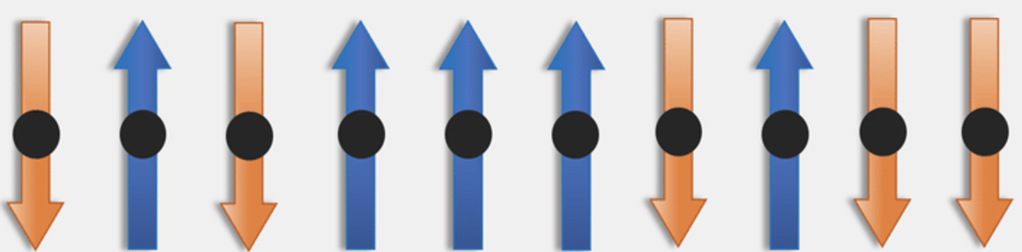
Given the local basis \(|\vec{\sigma}\rangle\in \{|\uparrow\rangle,|\downarrow\rangle\}\) then a basis state has the form:
\(|\vec{\sigma}\rangle=\) \(\left|\sigma_1,\sigma_2,\cdots,\sigma_{N-1},\sigma_N\right\rangle\)
There exists some generic quantum state \(|\Psi\rangle\) for the photon spin-\(\frac{1}{2}\) chain in this basis:
\(|\Psi\rangle=\sum_{\vec{\sigma}_n}^N C_{\vec{\sigma}_n}\left|\vec{\sigma}_n\right\rangle\)
When expressed in this form, the state \(|\Psi\rangle\) is called a MPS, or more broadly, a tensor network. This representation is exact, allowing any quantum state to be written this way, provided the bond-dimension \(\chi\), which is the shared index between the tensors, is large enough.
The complex, \(C_{\vec{\sigma}_n}\) tensor can is composed of rank-\(3\) tensors \(C_{\sigma_1, \cdots, \sigma_N}\) \(=A_{a_0, a_1}^{\sigma_1}, A_{a_1, a_2}^{\sigma_2}, \) \(\cdots, A_{a_{N-2}, a_{N-1}}^{\sigma_{N-1}}, A_{a_{N-1}, a_N}^{\sigma_N}\)
The contraction of matrices occurs over shared incdicies between rank-\(3\) tensors in the photon spin-\(\frac{1}{2}\) chain. This is because these shared indicies represent nearest-neighbor interactions between sites or particles. Given shared indicies are summed over, indicies \(a_{1},a_{N}\) are trivial \(1\)D indicies, and subscript indices are dropped because they are implied in matrix multiplication, the generic quantum state \(|\Psi\rangle\) can be written as:
\(|\Psi\rangle\) \(=\sum_{\sigma_1, \cdots, \sigma_N} A^{\sigma_1} A^{\sigma_2} \cdots A^{\sigma_{N-1}} A^{\sigma_N}\) \(\left|\sigma_1, \cdots, \sigma_N\right\rangle\)
Now, let's look at how we can decompose quantum states and express the state them as a MPS. One way to obtain a MPS representation of a quantum state is to use Schmidt decomposition \(N-1\) times. Note, that if the quantum circuit which prepares the many body state is given, than we can alternatively obtain a matrix product operator representation of the circuit, which we will look at later. Schmidt decomposition is done to reduce the degrees of freedom by identifying those that contain the most relevant information. Here, we will examine iterative reshaping of coefficient arrays and singular value decomposition SVD. Where SVD can correspond to the Schmidt decomposition for a properly reshaped array of state coefficients:
\(|\Psi\rangle\) \(=\sum_{s_1, \ldots, s_N} c^{s_1, \ldots, s_N}\left|s_1, \ldots, s_N\right\rangle\)
depending on the chosen bipartition of the lattice. The chosen bipartition is uniquely determined in the one dimension case with:
\(c^{s_1, \ldots, s_N} \rightarrow c^{\left(s_1, \ldots, s_\ell\right)},\) \(\left(s_{\ell+1}, \ldots, s_N\right)\) \(=\sum_{a_\ell} U_{a_\ell}^{\left(s_1, \ldots, s_\ell\right)} \Lambda^{a_\ell, a_\ell}\left(V^{\dagger}\right)_{a_\ell}^{\left(s_{\ell+1}, \ldots, s_N\right)}\)
where \(\Lambda\) is a diagonal matrix containing Schmidt coefficients \(\lambda_{a_{l}}\) and physical indices (\(\ldots\)) refer to matrix unfolding for tensors.
For a properly reshaped array of state coefficients for some state \(|\Psi\rangle\), given the following decomposition for rank-3 tensors \(A_{a_\ell}^{1,\left(s_1, \ldots, s_\ell\right)}\) \(=U_{a_l}^{\left(s_1, \ldots, s_\ell\right)}\) and \(B_{a_l}^{\left(s_{\ell+1}, \ldots, s_N\right), 1}\) \(=\left(V^{\dagger}\right)_{a_l}^{\left(s_{\ell + 1} \ldots, s_N\right)}\) we get:
\(|\Psi\rangle\) \(=\sum_{s_1, \ldots, s_N} \sum_{a_{\ell}} A_{a_{\ell}}^{1,\left(s_1, \ldots, s_{\ell}\right)} \Lambda^{a_\ell, a_\ell}\) \(B_{a_{\ell}}^{\left(s_{\ell+1}, \ldots, s_N\right), 1}\left|s_1, \ldots, s_N\right\rangle\) \(=\sum_{a_{\ell}} \lambda_{a_{\ell}}|a\rangle_{a_{\ell}}|b\rangle_{a_l}\)
which we can see illustrated in the figure below:
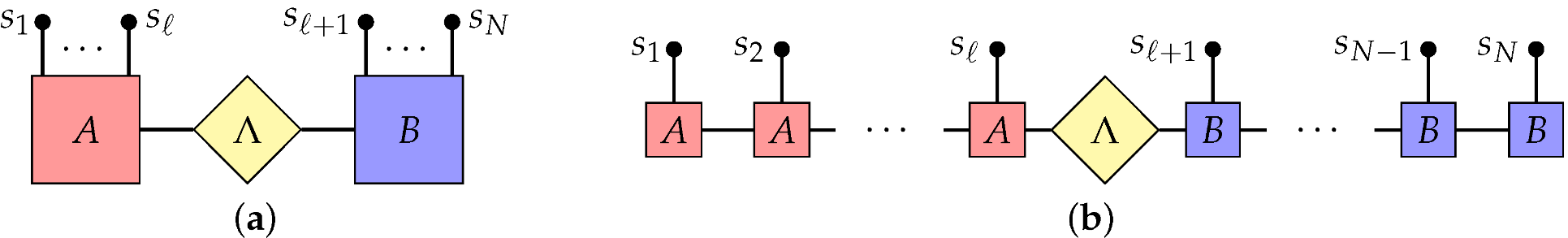
Image Source: https://www.mdpi.com/2673-8716/3/3/33
To continue.
Multi-scale Entanglement Renormalization Ansatz
Entanglement renormalization is a numerical technique that locally reorganizes the Hilbert space of a quantum many-body system to reduce entanglement in its wave function. It addresses computational challenges of real-space renormalization group RG methods, which struggle with the rapid growth of degrees of freedom that occur during successive transformations of RG transformations.
The key idea is that as a result of local character of physical interactions, some relevant degrees of freedom in the system's ground state of many-body system can be decoupled from the rest by applying unitary transformations called disentanglers to small regions, isolating and removing these degrees of freedom from the system, preventing their accumulation in future descriptions.
This approach enables more efficient real-space RG transformations, capable of handling large \(1\)D and \(2\)D lattice systems, even at quantum critical points. It also forms the basis for the MERA, a variational method for approximating many-body states. MERA is based on a class of quantum circuts and succesful at describing ground state at quantum criticality or topological order. A key property of MERA that we will focus on for QCNN is how, from a computiational perspective, MERA efficently optimizes its tensors based on the evalution of expected values of local observables.
More formally, let \(\mathcal{L}\) denote a \(D\)-dimensional lattice with \(N\) sites. Each site \(s_{1},...,s_{N} \in \mathcal{L}\) is a described by a Hilbert space \(\mathbb{V}\) of finite dimension \(d\), such that \(\mathrm{V}_{\mathcal{f}} \cong \mathrm{V}^{\otimes N}\). MERA is an ansatz used to describe certain pure states \(|\Psi\rangle \in \mathbb{V}_{\mathcal{L}}\) of lattice \(\mathcal{L}\), or of subspaces \(\mathbb{V}_U \subseteq \mathbb{V}_{\mathcal{L}}\).
Coarse-graining and Ground State Entanglement
As before, let's consider a quantum spin model described by a lattice \(\mathcal{L}\) in \(D\) spatial dimensions. Note, most derivations will involve a lattice on one spatial dimension, for simplicity, however, an important feature of entanglement renormalization ER is it applies to higher dimensional casses as well.
The goal is to compute low energy properties of the system, described as the ground state \(\left|\Psi_{\mathrm{GS}}\right\rangle \in \mathbb{V}^{\otimes N}\) of Hilbert space \(H\). Let \(o_1, o_2, \cdots, o_k\) be an arbitrary local operators acting on parts of the \(\mathcal{L}\). To predict how the system reacts to arbitrary external probes, we can use expected values of compute quantities such as:
\(\left\langle o_1 o_2 \cdots o_k\right\rangle_{\Psi_{\mathrm{GS}}}\) \(\equiv\left\langle\Psi_{\mathrm{GS}}\right| o_1 o_2 \cdots o_k\left|\Psi_{\mathrm{GS}}\right\rangle\)
We would like to continue this way, however, only very small systems can be computed by diagonalizing \(H\) for \(|\Psi_{\mathrm{GS}}\rangle\) like above, since the exponential growth in \(N\) of dimension \(\mathbb{V}^{\otimes N}\). Thus, to compute larger systems, we build a transformation that removes short-distance degrees of freedom from the lattice model \((\mathcal{L}, H)\) to narrow down on expected values that help predict how the system reacts to the arbitrary external probes. This initial lattice model is mapped into an effective lattice model \((\mathcal{L^{\prime}}, H^{\prime})\) such that:
\(\left\langle o_1^{\prime}, o_2^{\prime}, \cdots, o_k^{\prime}\right\rangle_{\Psi_{\mathrm{GS}}^{\prime}}\) \(=\left\langle o_1, o_2, \cdots, o_k\right\rangle_{\Psi_{\mathrm{GS}}}\)
where, \(|\Psi_{\mathrm{GS}}^{\prime}\rangle\) is the ground state of \(H^{\prime}\). The operators \(o_1^{\prime}, o_2^{\prime}, \cdots, o_k^{\prime}\) are a result from transforming \(o_1, o_2, \cdots, o_k\)
From above, we have a model \((\mathcal{L^{\prime}}, H^{\prime})\) that has a smaller Hilbert space dimension than the original model, thus making diagonalizing \(H^{\prime}\) mroe computationally affordable. Thus, larger models can be addressed.
With finite-size scaling techniques, the implication is that a powerful numerical route to study quantum critical phenomena is made possible with MERA. This can be used for coarse-graining transformation to remove short-distance degrees of freedom to investigate how \(H\) changes under scale transformations, and with RG help, evaluate the thermodynamic limit directly. However, for our purpose as MERA relates to QCNN, it is important to remember a QCNN is MERA inversed.
Quantum Convolutional Neural Network
Section Reference: Vidal, G. (2006, October 12). A class of quantum many-body states that can be efficiently simulated. arXiv. https://arxiv.org/abs/quant-ph/0610099 \(^{[1]}\)
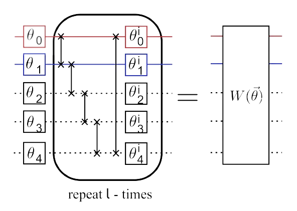
Consider a square lattice \(\mathcal{L}\) in \(D\) spatial dimensions with \(N\) sites, where each site \(s_{1},...,s_{N} \in \mathcal{L}\) is a complex vector space \(\mathbb{V}\) with finite dimension \(\chi\), termed the bond dimension. Site \(s\) can be described by a pure quantum state \(|\Psi\rangle \in \mathbb{V}^{\otimes N}=\mathbb{V}_\mathcal{L}\). This state is made of \(N\) quantum wires, which has a reduced density matrix \(\rho^{[s]}=\operatorname{tr}_{\bar{s}}(|\Psi\rangle\langle\Psi|)\). Unitary gates \(u\) transform the unentangled state state \(|0\rangle^{\otimes N}\) into state \(|\Psi\rangle\), which is be generated by a quantum circut \(\mathcal{C}\) with depth \(\Theta \equiv 2 \log _2(N)-1\). A figure of this quantum circut is given below:
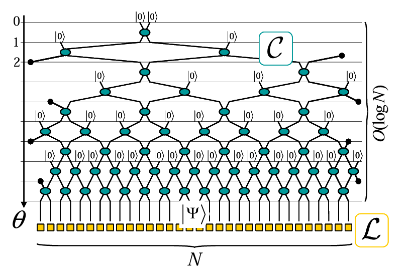
Image Source: \([1]\)
Generically, each unitary gate \(u\) in the circuit \(\mathcal{C}\) incoporates some small number \(p\) of wires.
To continue.